Cooperative Robot Localization with Vision-based Mapping

Cooperative Robot Localization with Vision-based Mapping ∗ Cullen Jennings

Don Murray

James J. Little

Computer Science Dept. University of British Columbia Vancouver, BC, Canada V6T 1Z4 {jennings,donm,little}@cs.ubc.ca Abstract Two stereo vision-based mobile robots navigate and autonomously explore their environment safely while building occupancy grid maps of the environment. A novel landmark recognition system allows one robot to automatically find suitable landmarks in the environment. The second robot uses these landmarks to localize itself relative to the first robot’s reference frame, even when the current state of the map is incomplete. The robots have a common local reference frame so that they can collaborate on tasks, without having a prior map of the environment. Stereo vision processing and map updates are done at 5Hz and the robots move at 200 cm/s. Using occupancy grids the robots can robustly explore unstructured and dynamic environments. The map is used for path planning and landmark detection. Landmark detection uses the map’s corner features and least-squares optimization to find the transformation between the robots’ coordinate frames. The results provide very accurate relative localization without requiring highly accurate sensors. Accuracy of better than 2cm was achieved in experiments.

1 Introduction Most robots that successfully navigate in unconstrained environments use sonar transducers or laser range sensors as their primary spatial sensors (for example, [1, 2]). While computer vision is often used with mobile robots, it is usually used for feature tracking or landmark sensing and seldom for occupancy grid mapping or obstacle detection. In this paper, we present a working implementation of a multi-robot navigation system that uses stereo vision-based robots. The robots use correlation-based stereo vision to map their environment with occupancy grids, which are ∗ This research was supported by grants from the Natural Sciences and Engineering Research Council of Canada and the Networks of Centres of Excellence Institute for Robotics and Intelligent Systems.

continuously updated to reflect the robot’s changing environment. The robots use the maps to navigate and autonomously explore unknown, dynamic indoor environments. We have also developed a method for detecting corners in the map and using them as landmarks. These landmarks are used to localize the robots with respect to one another. The robots can then safely share and cooperate within the same local environment. Our initial robot, Spinoza[3], demonstrated stereobased mapping and navigation. In [4], we presented algorithms for path planning and exploration using the generated map. In [5], we described in detail how to generate occupancy grid maps from stereo vision and how to compensate for various systematic errors specific to stereo vision in order to have a robust mapping system. This paper focuses on the localization problem of robust navigation. Localization is the problem of identifying the robot’s current position and orientation with respect to some common coordinate system. A robot in an unknown position must refer to its environment to determine its location. Even after localization, drift in odometry causes the estimated position to incrementally deviate from the true position. We present a landmark-based method for localizing within a local coordinate system. Localization is a difficult problem that has inspired several different approaches. One is to place distinctive, identifiable landmarks at known locations in the robot’s environment. This engineering solution is prohibitively expensive and generally difficult to justify outside hospitals or factories[6]. Another approach is to search the local environment for visually distinctive locations and record as landmarks these locations and a method to identify them (usually their visual appearance)[7]. Some systems concentrate on known types of visual events—finding vertical lines associated with doors, for example, or using range sensing, such as laser stripe systems, sonar, or active stereo vision to find locally salient geometric locations, such as corners, doors, or pillar/floor junctions. One can also track “corners”, local 2D image features, over sequences of image frames[8],

from which the 3D location of the corner points and the motion of the sensor can be determined[9]. Several working systems have been reported. Borthwick and Durrant-Whyte [10] base their system on detecting corner and edge features in 2D maps, using Extended Kalman Filtering to estimate both feature locations and robot position. Weckesser et al. [11] use a priori landmarks at known positions in the global coordinate frame and particular models for landmarks (such as door jambs). Their system uses active stereo cameras and can effectively solve for pose of the robot with respect to landmarks. Thrun and Bucken [12] base their system on sensing regular landmarks, such as overhead lights or doorways, rather than distinctive ones. It uses a Bayesian approach implemented in neural nets and learns which landmarks are most salient. Our system uses landmarks within the 2D map, as do Borthwick and Durrant-Whyte. Since the occupancy grids are the result of the integration of several sensor readings, features within the map tend to be more robust and less subject to noise than features in a single sensor reading. We divide our map into a series of local coordinate frames, each with a set of landmarks for localization within the local frame. When two robots are within the same “node” of the map, they can localize with the same landmarks and operate in a common coordinate system. Corner landmarks in the map are found with a leastsquares model fitting approach that fits corner models to the edge data in the map. These landmarks are found for both the reference map and the current map. A leastsquares approach then finds the transformation between the two maps based on matching the landmarks between the two. Section 2 describes the robots and how they build maps with stereo vision using occupancy grids. Section 3 shows how we detect corner features in the occupancy grids. Section 4 describes how we localize the robots given the landmark information. In section 5, we show the results of our localization approach. The final section concludes and describes future work.

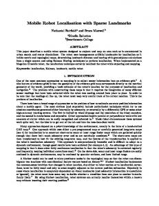
2 Mapping We used a RWI B-14 mobile robot, Jos´e, to conduct our experiments. Jos´e uses a Triclops trinocular stereo vision camera module.1 Jos´e’s partner, Eric, is identically equipped. The stereo vision module has 3 identical wide angle (90◦ degrees field-of-view) cameras. The environment is like a normal office: it is not highly textured and it has many right-angled corners. The hallway that produced the localization data is shown in Figure 1. 1 See

www.ptgrey.com.

Figure 1: Hallway near where map was localized

2.1 Occupancy grid mapping and stereo vision Occupancy grid mapping, pioneered by Moravec and Elfes [13, 14], is simple and robust, flexible enough to accommodate many kinds of spatial sensors, and adaptable to dynamic environments. It divides the environment into a discrete grid and assigns to each grid location a value related to the probability that the location is occupied by an obstacle. Sensor readings are used to determine regions where an obstacle is anticipated. The grid locations that fall within these regions have their values increased, while locations in the sensing path between the robot and the obstacle have their probabilities of occupancy decreased. Grid locations near obstacles thus tend to have a higher probability of being occupied than do other regions. Although occupancy grids may be implemented in any number of dimensions, most mobile robotics applications (including ours) use 2D grids. The stereo data provides 3D information that is lost in the construction of a 2D occupancy grid map. This reduction in dimension is justified because indoor mobile robots inhabit a fundamentally 2D world. The robot possesses 3 DOF (X, Y, heading) within a 2D plane corresponding to the floor. By projecting all sensed obstacles to the floor, we can uniquely identify free and obstructed regions in the robot’s space. Figure 2 shows the construction of the 2D occupancy grid sensor reading from a single 3D stereo image. Figure 2(a) shows the reference camera grayscale image (160x120 pixels). The resulting disparity image is shown in Figure 2(b). White regions indicate areas of the

(a)

(b)

(c)

(e)

(d)

Figure 2: From stereo images to top-down views: (a) grayscale image (b) disparity image (white indicates invalid, otherwise brighter indicates closer to the cameras) (c) the maximum disparity in each column of the disparity image (d) depth versus column graph (depth in centimeters) (e) the resultant estimate of clear, unknown and occupied regions (white is clear, black is occupied and gray is unknown)

image which were invalidated and thus not used. Darker areas indicate lower disparities, and are farther away from the camera. Figure 2(c) shows a column-by-column projection of the disparity image, taking the maximum valid disparity in each column. The result is a single row of maximum disparities, representing the closest obstacle in each column. Figure 2(d) shows these column values converted into distance, and (e) shows these distance values converted into an occupancy grid representation, with black indicating the uncertainty region around the object and white indicating regions that are clear. The two “spikes” in Figure 2(d) were caused by mismatches in the stereo algorithm; their causes and removal are discussed in [5]. The process illustrated in Figure 2 generates the input into our stereo vision occupancy grid. The mapping system then integrates these values over time, to expand the map and keep it current in the changing world. Although the map in Figure 3 looks like directions to buried treasure, it actually depicts our lab and nearby hallways.

Figure 3: Map generated over single run

3 Landmarks in Occupancy Grids We do localization using visual information stored in an occupancy grid, so we need to detect features in the map. Corners are appealing because they are distinctive, each constrain 2 degrees of freedom, occur frequently in indoor environments, and stand out well in occupancy grids despite quantization. There are many ways to detect features (correlation, Hough transform, Karhunen-Loeve Transform), but we chose a least-squares model matching approach because it is capable of subpixel resolution and is fast and trackable, meaning that if we have an estimate of the solution, we can use it to find the real solution. Once the landmarks are found, we match the landmarks in the two maps being considered to find the local coordinate transformation between the two maps.

3.1 Landmark Detection First we find boundaries between empty and solid spaces in the occupancy grid—we call these edges. Next, we find possible locations for corner models and use these as initial estimates. Third, we do a least-squares fit of a corner model to the map edge data to find all the corner landmarks.

Figure 4: Edges found in the occupancy grid (left), and the occupancy with landmarks found (right). 3.1.1 Finding edges in map Finding edges in occupancy maps is complicated by the fact that there is often a region of uncertainty between a region that is certainly occupied and one that is not. To overcome this we grow regions of certainty in the map into regions of uncertainty. Where we are highly confident that a certain region is empty or occupied, we mark these accordingly. We preserve the regions that have never been seen. Next we find occupied regions that are adjacent to empty regions and mark them as “edge” pixels. Models are fit directly to edge grid locations. Figure 4 shows the edges found by this process.

3.2

Model initialization

Our problem is finding initial estimates of possible locations that might fit a corner model. We start with the edge image. We dilate this several times and then compute an orientation map for each grid location—the ith bit is set if a line in the dilated edge map can extend for a fixed number of grid locations from this location in a direction of i×45◦ . Then we determine the corner map by looking within the orientation map for grid locations that have the ith and the (i + 2)th bits set. The search for a model fit is performed in the dilated edge map in order to save processing time. The dilated map has been dilated enough that a line at 22.5◦ dilates to an area that overlays a line at 0◦ for a length as long as the legs of the corners being matched. This guarantees that the orientation map will have a bit set if the model fits the edge data at any rotation.

3.3

Model fitting

The corner model is just two line segments of a fixed length (500mm in our case) that intersect at a 90◦ angle. The problem is to fit a model of a corner that is parameterized by X, Y, Θ to the edge grid locations, given an initial estimate of position and orientation.

The model of the corner is discretized into n points, labeled m1 , m2 , ..mn , which are evenly distributed along the model. Let x = [X, Y, θ]T . Now, the n points can be determined as a function of x, so mi = fi (x). Let x0 be the initial estimate of x. The error of the model at each point mi is the distance from mi to the nearest edge location. A Euclidean distance metric is used. These distances form the vector   dist(m1 , nearestedge),  dist(m2 , nearestedge),    e= .  .  .,  dist(mn , nearestedge), The vector e has the distance from each point to the nearest edge. The Jacobian, J, of e with respect to x is computed by evaluating the partial derivative of ∂dist(fi (x), nearestedge) ∂xj evaluated around the current estimate of x. Most of the time in localization is spent finding the nearest edge location to a given point while computing the Jacobian. Following the technique of Newton, the change in x from this estimate xi to the next estimate xi+1 is given by: J(xi+1 − xi ) This is an over-constrained system, since the model is discretized into n points, which make it much larger than the 3 DOF of the model. The least-squares solution to this is given by min ||J(xi+1 − xi ) − e||2 This is the same as solving the normal equations J T J(xi+1 − xi ) = J T e This model fitting works much better when this system of equations is stabilized by adding the constraint xi+1 − xi = 0 This constraint needs to be appropriately scaled in the least-squares solution, as shown by Lowe[15]. We measure position in grid cells and angle in degrees, and we scale all constraints equally by 0.1. This scaling indicates that we are willing to change the solution by 10 grid locations to avoid a 1 grid location error. Let the ma1 trix W be 10 I. The system to which we wish to find the least-squares solution becomes:     J e (xi+1 − xi ) = W 0

and the normal equations become (J T J + W T W )(xi+1 − xi ) = J T e

edges are shown in Figure 6 with the detected landmarks drawn as black corners and overlaid on the edges. The

These are solved with Gaussian elimination with pivoting on the optimal row. The system is run for 10 iterations or until the change from the previous iteration is very small. Convergence is fairly good, normally occurring after 3 iterations.

4 Localization 4.1

Corner Matching

The goal at this stage is to take two maps, the reference and current maps, and match the corners between them. First we eliminate all corner models with an RMS error above 1.5 pixels. (This is one of the few “magic numbers” in the system.) A corner will suppress all corners with a higher RMS error that are within 500mm of the suppressing corner. This non-maximal suppression reduces the chances of the corner being mismatched. Finally each corner is matched to the nearest corner in the other map. If no matching corner is found within 1000mm of a particular corner, the corner is left unmatched and not used for localization. Checking that the orientations of the corners matches does not seem to change the system’s robustness much. If there had been more mismatches, it would likely have helped.

Figure 5: Reference map from first robot

Figure 6: Edges and landmarks in reference map

4.2

Localization

The goal here is to find the transformation that maps the corners in one map to the other. This stage uses the same least-squares model matching technique that we used to match the corner models to the edges. The transform is parameterized by a 2D translation and rotation about the robot. The three parameters are found by setting up equations for each pair of landmarks that match between the maps. The rotation error between the maps is usually quite small (less than 15◦ ), so the linearization of the transform in the least-squares matching process introduces minimal error and the method quickly converges. The stabilization technique mentioned in Section 3.3 is important for nice convergence at this stage.

5

location of the robot when it acquired this map was marked so that it could be used as ground truth for comparing the location of the second robot. The second robot was run out to a nearby location and created the map shown in Figure 7. The associated edges and landmarks are shown in Figure 8.

Experiments

The first robot toured around our building creating the map shown in Figure 3. The intersection of two hallways (Figure 1) was selected as a localization node. The local occupancy map for this area is shown in Figure 5. The map

Figure 7: Current map from second robot The odometry estimates have drifted, as shown in Figure 9, which overlays the edges from the first and second

Figure 8: Edges and landmarks in current map robots. By comparing the locations of the two robots as marked on the floor, we know the length of the transformation between the reference frames should be 80 ± 20mm. The localization routine produced a transform of length 92mm.2 The transformation found was applied to the edges in the second map, and they were overlayed on the reference map from the first robot to get the image shown in Figure 10.

detect multiple corners very close together. Most of our corners are more than 1000mm apart. This ensures that for up to 500mm of odometry error, we are highly likely to match to the correct corner. Since the system finds naturally occurring corners in the environment, it can localize fairly often and have much smaller odometry errors between localizations. The technique can be used to localize a robot to a location that it has previously visited or that has been visited by another robot. It can also be used to localize two robots that are in the same space and need to share coordinate systems to collaborate on a task. The system is fast enough for real time robotics. The landmark detection for the image shown in this paper took 14 seconds running on a 266MHz Pentium II. Computing the localization took only a few milliseconds. The speed of this localization would allow for many possible transformation models to be tested and the best one chosen if needed. We did not find a need for this.

6 Conclusions and Future work

Figure 9: Edges of two maps overlayed before localization

Figure 10: Edges of two maps overlayed after correction for localization The system is quite robust and correctly localizes the robot in a wide variety of situations. It starts to fail where the odometry estimate is so far out that the corners are mismatched. By using fairly large corners (500mm per side) and non-maximal suppression we ensure that we do not 2 In the final paper we plan to do additional test runs and gather some statistics relating the ground truth and localization results

This paper demonstrates a working system in which robots can localize themselves relative to other robots or to themselves at other times. The system is very accurate and works with incomplete maps of environments that are being explored. It was shown that localization using features in stereo vision occupancy grids is a feasible solution to the mobile robot localization problem. Accuracy better than a few centimeters are attainable in real time. Our corner localization works well because we base the localization on data integrated over several views, a method more robust than a single reading would be. We can also extend the landmark detection method to use ’multi-level’ 2D maps. These are collections of 2D slices of the 3D environment. Near ceilings, room corners are rarely obstructed and are readily apparent. These can be used as commonly occurring landmarks. Further, a more comprehensive cooperative mobile robot environment could be built relying on the groundwork presented here. A group of landmarks can form a local coordinate frame, and locally consistent frames can be linked so as to create nodes useful for developing topological maps. Exploration of the environment can also be a cooperative task, with one robot altering its behavior in response to its partner’s activities. These and other related ideas would be suitable topics for future work.

Acknowledgments Special thanks to Rod Barman, Stewart Kingdon, David Lowe, and the rest of the Robot Partners Project.

References [1] G. Dudek, M. Jenkin, E. Milios, and D. Wilkes, “On building and navigating with a local metric environmental map,” in ICAR-97, 1997. [2] W. Burgard, A. B. Cremers, D. Fox, D. H¨ahnel, G. Lakemeyer, D. Schulz, W. Steiner, and S. Thrun, “The interactive museum tour-guide robot,” in AAAI98, pp. 11–19, 1998. [3] V. Tucakov, M. Sahota, D. Murray, A. Mackworth, J. Little, S. Kingdon, C. Jennings, and R. Barman, “Spinoza: A stereoscopic visually guided mobile robot,” in Proceedings of the Thirteenth Annual Hawaii International Conference of System Sciences, pp. 188–197, Jan. 1997. [4] D. Murray and C. Jennings, “Stereo vision based mapping for a mobile robot,” in Proc. IEEE Conf. on Robotics and Automation, 1997, May 1997. [5] D. Murray and J. Little, “Interpreting stereo vision for a mobile robot,” in IEEE Workshop for Perception for Mobile Agents, pp. 19–27, June 1998. [6] S. B. Nickerson et al., “Ark: Autonomous navigation of a mobile robot in a known environment,” in IAS-3, pp. 288–293, 1993. [7] S. Oore, G. Hinton, and G. Dudek, “A mobile robot that learns its place,” Neural Computation 9, pp. 683– 699, Apr. 1997. [8] J. Shi and C. Tomasi, “Good features to track,” in Proc. IEEE Conf. Computer Vision and Pattern Recognition, 1994, pp. 593–600, 1994. [9] C. Tomasi and T. Kanade, “Factoring Image Sequences into Shape and Motion,” in Proc. IEEE Workshop on Visual Motion, 1991, pp. 21–28, IEEE, 1991. [10] S. Borthwick and Durrant-Whyte, “Simultaneous localisation and map building for autonomous guided vehicles,” in IROS-94, pp. 761–768, 1994. [11] P. Weckesser, R. Dillmann, M. Elbs, and S. Hampel, “Multiple sensorprocessing for high-precision navigation and environmental modeling with a mobile robot,” in IROS-95, 1995. [12] S. Thrun and A. Bucken, “Learning maps for indoor mobile robot navigation,” tech. rep., CMU-CS-96121, Apr. 1996. [13] H. Moravec and A. Elfes, “High-resolution maps from wide-angle sonar,” in Proc. IEEE Int’l Conf. on Robotics and Automation, (St. Louis, Missouri), Mar. 1985. [14] A. Elfes, “Using occupancy grids for mobile robot perception and navigation,” Computer 22(6), pp. 46– 57, 1989.

[15] D. G. Lowe, “Fitting Parameterized Three-Dimensional Models to Images,” IEEE Transactions on Pattern Analysis and Machine Intelligence 13, pp. 441–450, May 1991.