Experiments with Underwater Robot Localization and Tracking

Experiments with Underwater Robot Localization and Tracking Peter Corke† , Carrick Detweiler∗ , Matthew Dunbabin† , Michael Hamilton◦ ,Daniela Rus∗ and Iuliu Vasilescu∗ †

Autonomous Systems Lab CSIRO ICT Centre Brisbane, Australia

∗

Computer Science & Artificial Intelligence Lab Massachusetts Institute of Technology Cambridge, MA 02139, USA

Abstract— This paper describes a novel experiment in which two very different methods of underwater robot localization are compared. The first method is based on a geometric approach in which a mobile node moves within a field of static nodes, and all nodes are capable of estimating the range to their neighbours acoustically. The second method uses visual odometry, from stereo cameras, by integrating scaled optical flow. The fundamental algorithmic principles of each localization technique is described. We also present experimental results comparing acoustic localization with GPS for surface operation, and a comparison of acoustic and visual methods for underwater operation.

I. I NTRODUCTION Performing reliable localization and navigation within highly unstructured underwater environments is a difficult task. Knowing the position and distance an Autonomous Underwater Vehicle (AUV) has moved is critical to ensure that correct and repeatable measurements are being taken for reef surveying and other applications. A number of techniques are used, or proposed, to estimate vehicle motion which can be categorized as either acoustic or vision-based. Leonard et al. [1] provide a good survey of underwater localization methods. Acoustic sensors such as Doppler velocity logs are a common means of obtaining accurate motion information, measuring speed with respect to the sea floor. Position can be estimated by integration but will be subject to unbounded growth in error. Long Base Line (LBL) systems employ transponder beacons whose position is known from survey, or GPS if they are on the surface. The vehicle periodically pings the transponders and estimates its position based on the round trip delay. Ultra Short Base Line (USBL) systems determine the angle as well as distance to a beacon. The largest source of uncertainty with this class of methods is the speed of sound underwater which is a complex function of temperature, pressure and salinity. A number of authors have investigated localization using vision as a primary navigation sensor for robots moving in 6DOF, for example Amidi [2] provides an early and detailed investigation into feature tracking for visual odometry for an autonomous helicopter, and Corke [3] describes the use vision for helicopter hover stabilization. The use of vision underwater has been explored for navigation [4] and station keeping [5], [6]. Dagleish presents a survey of vision-based underwater vehicle navigation for the tracking of cables, pipes and fish [7], and for station-keeping and positioning [8]. Of critical importance in these systems is the longterm stability of the motion estimate. Current research is

◦

University of California James San Jacinto Mountains Reserve Idyllwild, CA 92549, USA

thus focusing on reducing motion estimation drift in long image sequences through techniques such as mosaicing and SLAM. Many examples are presented, but most algorithms were only applied to recorded data sets or implemented on an ROV allowing significant computing power, not on an energy-constrained AUV. Each method above has different advantages and disadvantages. Visual odometry, by its nature integrates perceived motion and is subject to long-term drift, and requires occasional “position fixes” to keep error in check. The acoustic localization system involves the creation of infrastructure which must be powered, but provides absolute position estimates. Complementary or hybrid systems could be created that would exploit the advantages of each method, but are not the subject of this paper. In this paper we compare, for the first time, these two quite different underwater localization methods. Our acoustic localization system is able to self calibrate the location of the static nodes, and then provide location information to the underwater vehicle. We compare the vehicle locations measured by the acoustic system with GPS during surface operations. In previous work it has been difficult to ground truth the visual odometry system since it requires close proximity to the sea floor, whereas as GPS requires operation at the surface. In this work we compare the dead reckoned location, from visual odometry, with the estimate from the acoustic localization system. We present experimental results from a recent ocean trial. The remainder of the paper is organized as follows. We describe the experimental platforms and procedures, and then present results for the acoustic and vision systems. Finally we compare the two methods and conclude. II. E XPERIMENTAL S TUDY A. Experimental Platforms 1) Sensor Nodes: The sensor nodes shown in Figure 1 were developed at MIT. These nodes package communication, sensing, and computation in a cylindrical water-tight container of 6in diameter and 10in height. Each unit includes an acoustic modem we designed and developed. The system of sensor nodes is self-synchronizing and uses a distributed time division multiple access (TDMA) communications protocol. The system is capable of ranging and has a data rate of 300 b/s verified up to 300 m in fresh water and in the ocean. Each unit also includes an optical modem implemented using

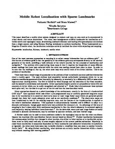
Fig. 1.

The sensor nodes drying in the sun.

green light. The sensors in the unit include temperature, pressure, and camera with inputs for water chemistry sensors. The sensor nodes differ from traditional LBL networks in a number of ways. First, the acoustic modems allow bidirectional communication. This allows the dissemination of range information to neighbors. The nodes obtain ranges using three different methods. When node A sends a message to B and B responds, A measures the round-trip time of the message to compute the range. The second method is for a node A to broadcast a range-request message to which all nodes in communication range respond at specific intervals thereafter. Using the round-trip times, ranges to all responding nodes are computed. The third method is to use onboard synchronized clocks and for nodes to ping at specified intervals. Listening nodes then compute the range based on the difference in the expected arrival time and the actual arrival time. Using this range information we are able to self-localize the static network using a 3D distributed localization algorithm based on work by Moore et al. [9]. This makes deployment extremely easy, the nodes can just be thrown overboard. The network localization information can also be transmitted to the mobile node to allow efficient localization and tracking of the mobile node within the network. Our network also allows multiple mobile nodes to be localized concurrently within the network. This is not possible in an LBL network. Unlike LBL networks we do not obtain range measurements simultaneously (or nearly so) as the bidirectional communication prevents this. Thus, we must compensate for the non-simultaneous ranges algorithmically. Additionally, our network is scalable to many nodes, whereas traditional LBL systems typically have just 4 beacons. This allows us to cover kilometer-scale areas despite the subkilometer range of our acoustic communication. 2) AMOUR: Autonomous Modular Optical Underwater Robot (AMOUR), Figure 2 , is an AUV developed at MIT. It has on-board computation, storage, batteries, and acoustic and optical communication. Its key performance specifications are: mass (11 kg), length 43.3 cm, diameter 15.3 cm, maximum forward thrust 70 N, maximum linear speed 1 m/s, maximum rotation speed 360 deg/s, and en-

Fig. 2.

AMOUR in Moorea with sensors in the background.

Fig. 3.

Deploying Starbug in Moorea.

durance 10 hours using lithium polymer battery. It has four external thrusters with a maximum power of 150 W and a maximum static thrust of 35 N each. Two thrusters act vertically and two thrusters act horizontally to provide forward-backward propulsion and yaw control. The bottom cap of the robot has a cone shaped cavity, designed for maximum mechanical reliability in docking and for optical communication. 3) Starbug: Starbug, Figure 3, is a hybrid AUV developed at CSIRO[10]. It has a powerful onboard vision system. Its key performance specifications are: mass 26 kg, length 1.2 m (folding to 0.8 m for transport), maximum forward thrust 20 N, maximum speed 1.5 m/s, and maximum endurance of 3.5 hours (8 km at 0.7 m/s) with current lead-acid battery technology. The vehicle is fully actuated with six thrusters providing forward, lateral and vertical translations as well as yaw, roll and pitch rotations. The vehicle’s drag and thrust characteristics were empirically determined leading to a simple still-water hydrodynamic model. Differences between the predicted vehicle motion based on actual control inputs and the instantaneous motion estimate from the vision system, allow the magnitude and direction of the water current to be estimated.

Starbug has two stereo vision heads: one looking downward for sea-floor altitude and speed estimation as well as mapping, and the other looking forward for obstacle avoidance. All cameras have firewire interface, with 640 × 480 pixel resolution in raw Bayer mode. Each stereo pair has a baseline of 70 mm which allows an effective distance resolution in the range 0.2 to 1.7 m. In addition to the vision sensors, the vehicle has a magnetic compass, custom built IMU (see [10] for details), pressure sensor (2.5 mm resolution), a PC/104 1.6GHz Pentium-M processor stack running Timesys Linux, and a tail-mounted GPS which is used when surfaced. By comparison, and by design, AMOUR is inexpensive and does not have an inertial measurement unit (IMU) or powerful computer. Instead it relies on the range measurements to the sensor nodes to determine its trajectory through the water. One of the design goals of Starbug has been to create a perceptually powerful robot using vision and low-end inertial sensing. The following experiments have been designed to compare and contrast the robots’ ability to localize in water using these two very different approaches. Both robots have the acoustic and optical communication capabilities of the static sensor nodes, which is accomplished by connecting each robot to a sensor node using a robotspecific communication protocol. B. Experimental Site During June 2006 we traveled to the University of California Berkeley Richard B. Gump South Pacific Research Station1 to run field experiments with AMOUR, Starbug and the acoustic sensor nodes. The Gump station is located in the South Pacific on the island of Moorea, near Tahiti in French Polynesia. We performed experiments in the inner reef waters off the coast of Moorea, north west of Cook’s Bay. The area we used was a hundred meter squared area with an average depth of four meters. C. Experimental Methodology The sensor nodes and the robots were deployed manually from a boat. The sensor nodes were anchored with dive weights of about 3kg. The location of the nodes was marked using red floats. The nodes self-localized and for ground truth the location of each node was recorded using GPS at deployment. One node was attached beneath Starbug’s hull and suitably ballasted to allow the robot to dive. The node has a large cross sectional area which adds significant drag, and the additional height must be taken into account when setting the terrain following altitude. One of the static nodes was connected by a serial data tether to a laptop computer on the boat allowing the status of the system to be monitored. The node on Starbug was connected via a serial data link to the onboard computer. Every two seconds the node obtained range measurements to 1 http://moorea.berkeley.edu/index.html

some of the nodes in the network, and the result was logged, along with other navigation and system status information, to the onboard hard disk. D. Location by Acoustic Tracking In previous work, [11], we developed a theoretical foundation for a passive tracking and localization algorithm. This previous work introduces the algorithm, presents correctness and complexity analyses, and simulation results. Building a real sensor-network system that implements this algorithm onto a distributed underwater sensor network subject to localization errors and communication uncertainty is a significant challenge. The contribution of this paper includes the engineering of a distributed version of the tracking and localization algorithm that runs on a physical underwater sensor network and extensive experimentation with this system. The rest of the section summarizes the algorithm in [11], discusses the challenges with creating a physical system that is based on this algorithm, and presents experimental data from the resulting implementation. There are a number of challenges associated with acoustic localization underwater. The acoustic channel is very narrow and low bandwidth. We are only able to communicate at 300 b/s. Thus, our localization algorithm must use a minimal amount of transmitted data. Due to the limits of the acoustic channel we are also only able to obtain non-simultaneous range measurements between nodes every couple of seconds. Therefore, our algorithm also has to deal with the potentially large motion of the robot between range measurements. Our approach is based on a field of statically fixed nodes that communicate within a limited distance and are capable of estimating ranges to neighbors. A mobile node moves through this field, passively obtaining non-simultaneous ranges to nearby fixed nodes and listens to broadcasts from the static nodes. Based on this information, and an upper bound on the speed of the mobile node, our algorithm recovers an estimate of the path traversed. As additional measurements are obtained, this new information is propagated backwards to refine previous location estimates, allowing accurate estimation of the current location as well as previous states. The algorithm takes a geometric approach and handles large motions of the robot between the non-simultaneous range measurements. Each range measurement forms an annulus/circle which represents the current location of the robot. As the robot moves through the water the annulus is expanded to account for the possible motion. Intersecting these regions produces a location estimate. We prove in [11] that the regions found are optimal localization regions–that is, the smallest regions that must contain the mobile node. Algorithm 1 shows the pseudocode for the acoustic localization algorithm. In practice it is run online by omitting the outer loop (lines 4-6 and 11) and executing the inner loop whenever a new region/measurement is obtained. The first step in Algorithm 1 (line 3), is to initialize the first intersection region to be the first region. Then we iterate through each successive region.

Algorithm 1 Localization Algorithm 1: procedure L OCALIZE (A1 · · · At ) 2: s ← max speed 3: I1 = A1 . Initialize the first intersection region 4: for k = 2 to t do 5: 4t ← k − (k − 1) 6: Ik =Grow(Ik−1 , s4t) ∩ Ak . Create the new intersection region 7: for j = k − 1 to 1 do . Propagate measurements back 8: 4t ← j − (j − 1) 9: Ij =Grow(Ij+1 , s4t) ∩ Aj 10: end for 11: end for 12: end procedure Fig. 4. The GPS data compared to the recovered path. The blue stars indicate the location of the static nodes, the black line is the GPS path and the red line is the recovered path.

The new region is intersected with the previous intersection region grown to account for any motion (line 6). Finally, the information gained from the new region is propagated back by successively intersecting each optimal region grown backwards with the previous region, as shown in line 9. For more details and analysis see [11]. 1) Experimental Results: The sensor nodes automatically localized themselves using a distributed static node localization algorithm we developed based on work by Moore et al. [9]. We used Starbug’s tail mounted GPS to provide us with ground-truth data and a sensor node to collect the acoustic ranging information. The experimental setup closely resembled the theoretical and simulation setup in all but a few aspects. In the theoretical work we assumed we knew the location of the static nodes exactly. In the experimental setup we had to determine the location using the static localization algorithm which could introduce errors into the calculation. Additionally, our proofs of optimality assumed that the range measurement ± the error always contained the true measurement. In our previous work we showed in simulation that violating this assumption did not greatly impact the performance of the algorithm. These experiments confirm that this is true given our real world data which contains outliers. We also used a limited back propagation time, as discussed in our previous work, to achieve constant runtime per update. The result of running the localization algorithm on the data we collected is compared to the GPS track in Figure 4. This shows that the algorithm performed well. The mean error was 0.6 m and the maximum error was 2.75 m. This is well within the noise bounds associated with the GPS. Additional experiments were performed with four sensor nodes localizing and tracking the AMOUR robot at Lake Otsego in New York State during September, 2006. Figure 5 shows the data collected during a 15 minute run of the passive location algorithm over an 80 × 80 meter area of the lake that is 20 meters deep. The nodes were deployed to float between 3 and 5 meters below the water surface. The nodes were localized using our distributed localization algorithm. Amour moved autonomously across this area on the surface

Fig. 5. Results from a 15 minute experiment with Amour in a lake. The red dashed line corresponds to the path traveled by Amour as recorded by a GPS unit. The blue solid like corresponds to the location path computed from ranges. The location of the sensor nodes is marked by *.

of the water. It collected both GPS and range information as it moved. We commanded the robot to move using its entire speed range during this experiment. The mean location error for Amour was 2.5 meters (which is within the noise of the GPS). E. Location by Vision Starbug was designed for coral reef environments which feature rich terrain, relatively clear shallow waters and sufficient natural lighting for which vision is a very well suited. The fundamental building block of our visual odometry system is the Harris feature detector which was chosen for its speed and satisfactory temporal stability for outdoor applications. Only features that are matched both in stereo (spatially) for height reconstruction, and temporally for motion reconstruction are considered for odometry estimation. Typically, this means that between ten and fifty strong features are tracked at each sample time.

For stereo matching, the correspondences between features in the left and right images are found. The similarity between the regions surrounding each corner is computed (left to right) using the normalized cross correlation similarity measure (ZNCC), and validation (right to left matching) is also implemented. Approximate epipolar constraints are used to prune the search space and only the strongest corners are evaluated. For each match the feature location is refined with sub-pixel interpolation and then corrected using the lens distortion model — we choose this order since the low-power processor does not have the cycles to undistort the original image. The tracking of features temporally between image frames is similar to the spatial stereo matching as discussed above but without the epipolar constraint. Motion matching is currently constrained by search space pruning, whereby feature matching is performed within a disc of specified radius about the image location predicted by motion at the previous time step (a constant velocity motion model). Our temporal feature tracking only has a one frame memory which reduces problems due to appearance change over time. A sophisticated multi-frame tracker such as KLT would be advantageous but is beyond the capability of our processor. Differential image motion (du,dv) is then calculated in both the u and v directions on a per feature basis. A 3-way match is a point in the current left image which is matched to a point in the right image and also the previous left image. Standard stereo reconstruction methods are then used to estimate a feature’s three-dimensional position. Since it cannot be assumed that a flat ground plane exists (as in [3]), the motion of the vehicle is predicted using an iterative least median squares method developed to estimate a six degree of freedom pose vector which best describes the translation and rotation of a set of 3D reconstructed points from the previous to the current frame. We formulate the problem as one of optimization to find at time k a vehicle rotation and translation vector (xk ) which best explains the observed visual motion and stereo reconstruction as shown in Fig. 6.

The differential motion vectors are then integrated over time to obtain the overall vehicle motion position vector at time tf such that xtf =

tf X

THk dxk

(1)

k=0

The Pentium-M processor currently updates odometry at 10 Hz. More details are provided in [4].

Fig. 7. (blue).

Comparison of demanded robot path (red) and estimated path

Figure 7 shows the demanded and estimated actual path of the Starbug robot during one of the Moorea trials, and several features deserve discussion. The robot is traveling clockwise around the circuit and on the left hand edge is moving into a very strong current. The vehicle’s control strategy is based on pure-pursuit of a target whose position is moved at constant speed by the vehicle’s mission planner. However, due to the strong water current at the test location, the maximum thrust was insufficient to match speed with the pursuit target. Hence, at the end of that path segment, the vehicle was almost 5m behind the target position. It then cut the corner on the next leg to catch the pursuit target, and performed very well when traveling with the current on this final segment. Along the bottom edge Starbug’s visual odometry system is very effectively rejecting the sideways thrust due to the water current. F. Comparison

Fig. 6.

Odometry optimization scheme.

In previous work it has been difficult to ground truth the visual odometry system since it requires close proximity to the sea floor, whereas GPS requires operation at the surface. In Figure 8 we compare the paths estimated by visual odometry and acoustic localization. The visual odometer has a cumulative error of just less than 5m error at the end of the 100 m transect or 5% of along track distance. Growth in error with distance traveled is expected with any odometry system. Figure 9 shows more details about the operation of the visual odometry system. The first trace is the depth as measured by the pressure sensor, the second trace is the

III. C ONCLUSIONS Knowing the position and distance a AUV has moved is critical to effective operation, but reliable localization and navigation within highly unstructured underwater environments is a difficult task. In this paper we compare, for the first time, two quite different underwater localization methods: acoustic localization and visual odometry. Our acoustic localization system is able to self calibrate the location of its static nodes, and then provide location information to the underwater vehicle. The localization accuracy is better than 2.5 m and comparable with GPS. The dead reckoned location, from visual odometry, shows a performance of 5% of along track error compared to the acoustic localization system. Our experiments were conducted in lake and ocean environments. Fig. 8. Comparison of acoustic estimated path (red) and vision estimated path (blue).

ACKNOWLEDGMENT Support for this work has been provided in part by NSF, Intel, the ONR PlusNet project, and the MIT-CSIRO alliance. We are very grateful for this support. The field experiments were done at the Richard B. Gump South Pacific Research Station and were supported by a grant from the NSF award 0120778 to the Center for Embedded Networked Sensing (CENS) and to the UC James San Jacinto Mountains Reserve. We are grateful to Neil Davies and Frank Murphy for their local support. R EFERENCES

Fig. 9. Comparison of demanded robot path (blue) and vision estimated path (red).

vision-based altitude estimation. The points that drop to zero altitude indicate when there are insufficient features for a reliable position estimate. In this situation the motion estimate is taken to be the same as the previous time step. The third trace is the magnitude of the estimated water current based on the difference between how the robot is trying to move based on the commanded thrusts and its internal hydrodynamic model, compared to the vision system estimate. This may be overestimated as the drag coefficient of the robot did not take into account the fact we had a large acoustic node strapped to the bottom of the robot. The final trace is the number of 3-way matches detected by the vision system and is an indication of seafloor texture.

[1] J. J. Leonard, A. A. Bennet, C. M. Smith, and H. J. S. Feder, “Autonomous underwater vehicle navigation,” MIT Marine Robotics Laboratory, Technical Memo 98-1, 1998. [2] O. Amidi, “An autonomous vision-guided helicopter,” Ph.D. dissertation, Dept of Electrical and Computer Engineering, Carnegie Mellon University, Pittsburgh, PA 15213, 1996. [3] P. Corke, “An inertial and visual sensing system for a small autonomous helicopter,” Journal of Robotic Systems, vol. 21, no. 2, pp. 43–51, Feb. 2004. [4] M. Dunbabin, K. Usher, and P. Corke, “Visual motion estimation for an autonomous underwater reef monitoring robot,” in Field and Service Robotics: Results of the 5th International Conference, P. Corke and S. Sukkariah, Eds. Springer Verlag, 2006, vol. 25, pp. 31–42. [5] S. van der Zwaan, A. Bernardino, and J. Santos-Victor, “Visual station keeping for floating robots in unstructured ennvironments,” Robotics and Autonomous Systems, vol. 39, pp. 145–155, 2002. [6] P. Rives and J.-J. Borrelly, “Visual servoing techniques applied to an underwater vehicle,” in Proceedings of the 1997 IEEE International Conference on Robotics and Automation, April 1997, pp. 1851–1856. [7] F. Dalgleish, S. Tetlow, and R. Allwood, “Vision-based navigation of unmanned underwater vehicles: a survey part 1: Vision-based cable-, pipeline-, and fish tracking,” Journal of Marine Design and Operations, no. B7, pp. 51–56, 2004. [8] ——, “Vision-based navigation of unmanned underwater vehicles: a survey part 2: Vision-based station-keeping and positioning,” Journal of Marine Design and Operations, no. B8, pp. 13–19, 2005. [9] D. Moore, J. Leonard, D. Rus, and S. Teller, “Robust distributed network localization with noisy range measurements,” in Proc. 2nd ACM SenSys, Baltimore, MD, November 2004, pp. 50–61. [Online]. Available: citeseer.ist.psu.edu/moore04robust.html [10] M. Dunbabin, P. Corke, and G. Buskey, “Low-cost vision-based AUV guidance system for reef navigation,” in Proceedings of the 2004 IEEE International Conference on Robotics & Automation, April 2004, pp. 7–12. [11] C. Detweiler, J. Leonard, D. Rus, and S. Teller, “Passive mobile robot localization within a fixed beacon field,” in Proceedings of the International Workshop on the Algorithmic Foundations of Robotics, New York, New York, 2006.