CPU Load Predictions on the Computational Grid - CiteSeerX

CPU Load Predictions on the Computational Grid * Yuanyuan Zhang1, Wei Sun1 and Yasushi Inoguchi2 1 Graduate School of Information Science, 2 Center for Information Science, Japan Advanced Institute of Science and Technology 1-1 Asahidai, Nomi, Ishikawa, 923-1292, Japan {yuanyuan, inoguchi, sun-wei}@jaist.ac.jp

Abstract The ability to accurately predict future resource capabilities is of great importance for applications and scheduling algorithms which need to determine how to use time-shared resources in a dynamic grid environment. In this paper we present and evaluate a new and innovative method to predict the one-stepahead CPU load in a grid. Our prediction strategy forecasts the future CPU load based on the tendency in several past steps and in previous similar patterns, and uses a polynomial fitting method. Our experimental results demonstrate that this new prediction strategy achieves average prediction errors that are between 37% and 86% lower than those incurred by the previously best tendency-based method.

1. Introduction Grid computing [1], the internet-based infrastructure that aggregates geographically distributed and heterogeneous resources to solve largescale problems, is becoming increasingly popular because it provides us with the ability to dynamically link resources together as an ensemble, to support the execution of large-scale, resource-intensive, and distributed applications. Task scheduling of the applications is an important component for achieving high performance in a grid computing environment, while the prediction of execution time of every application is one of the most important elements in determining such scheduling. The execution time of a CPU-bound task on a host is tightly related to the CPU load on the host. In fact, * This research is conducted as a program for the "21st Century COE Program" by Ministry of Education, Culture, Sports, Science and Technology, Japan. P

for some applications the relationship between the execution time of a CPU bound task and the measured load during the execution is almost perfectly linear [2]. If we could predict the load during the execution of a task on a host, we could predict easily the execution time of the task on the host. Therefore, host load prediction can be useful for guiding scheduling strategies to achieve high application performance and efficient resource use [3]-[6]. However, in a grid environment, since applications compete for resources with unknown workloads from other users, resource contention causes host load and availability to vary over time, and makes the load prediction problem more difficult. In this paper we propose a new one-stepahead time series prediction strategy that behaves better than previously proposed techniques. Our prediction strategy is a kind of tendency-based method. However, the difference between our method and the conventional tendency-based method proposed by Yang [7] is that they predicted according to the “ascending” or “descending” tendency one-stepbackward, and used linear increments, while our method predicts the one-step-ahead load based on the tendency several steps backward, and uses a 2nd or 3rd polynomial fitting method to produce the prediction value. We also conduct the prediction based on a search of previous similar “patterns”. Our experimental results on a commonly used host load measurement dataset show that our proposed strategy consistently outperforms the previous tendency-based predictor, which in turn has been proved to behave better than the Network Weather Service (NWS) [8]-[11], a widely used performance prediction system. The rest of the paper is structured as follows. Section 2 introduces background and related work. Section 3 describes our prediction strategy in detail. Section 4 describes the results of an experiment in which our prediction method was applied to realistic

load measurements and compared with previous work. Finally in Section 5 we conclude the paper.

2. Background and related work In [12] Dinda provided a comprehensive analysis, including summary statistics, distributions, and time series analysis, on the statistical properties of a host load. The significant result is that the load exhibits complex properties such as self-similar and epochal behavior, but is still consistently predictable to a very useful degree from past behavior. This work encourages us that there is abundant opportunity for prediction algorithms to improve matters. Several prediction strategies for the CPU load in the grid environment have been proposed by researchers working on this field [13][14]. Among them, NWS is a distributed system that periodically monitors and dynamically forecasts the performance of network and computational resources over a given time interval. For every resource, NWS uses various predictive methods to forecast simultaneously. The method exhibiting the best overall predictive performance at any time t is then used to generate the forecast of the measurement at time t+1. The predictive methods currently used in NWS include running average, sliding window average, last measurement, adaptive window average, median filter, adaptive window median, α-trimmed mean, stochastic gradient, and autoregression. Dinda et al. [2] evaluated different linear time series models [15], including AR, MA, ARMA, ARIMA, and ARFIMA, for predicting loads from 1 to 30 seconds into the future. His conclusion is that considering both overhead and prediction accuracy, simple, practical models such as AR are sufficient for host load prediction. In [7] Yang et al. proposed several homeostatic and tendency-based one-step-ahead prediction strategies. Homeostatic methods are based on the assumption that the mean of a time series remains steady, while tendency-based strategies assume the time series always retains its “tendency”, that is, if current value increases, the next value will also increase, or vice versa. The increment/decrement value used in the methods is adjusted according to the magnitudes of the last load measurement and the last prediction error. It is shown that this technique outperforms the commonly used methods in NWS for CPU load predictions. In this paper we propose a new one-step-ahead load prediction strategy. Our strategy is a kind of tendency-based method; however, the difference between our method and the tendency-based method

described in [7] is that [7] predicts according to the tendency one step backward, and uses linear increment, while our method predicts the one-step-ahead load based on the tendency several steps backward, and uses polynomial fitting to produce the prediction value. We also predict based on the measured loads of previous similar “patterns”.

3. CPU load prediction This section describes our prediction strategy. Based on our study on the statistical properties of host load traces, our one-step-ahead prediction strategy predicts the next load value based on polynomial fitting method and “similar” patterns. We use the following notations in the description of the prediction strategy: VT: the measured load at the Tth measurement. PT+1: the predicted load for the (T+1)th measurement. N: number of historical data points used for the prediction of PT+1.

3.1. Polynomial fitting In scientific experiments, it is often necessary to disclose the relationship between the independent variable x and the dependent variable y from a set of experimentally observed data (xi, yi), I = 0, 1, …. Such a relationship usually can be approximately expressed by the function: y = f(x). One method to produce function f(x) is a Least Squares Polynomial Fitting, which can be expressed as follows: Given a discrete sampling of N data points D1, D2, … DN which have coordinates (i = 1,2,…, N) (1) Di = (xi, yi) it is assumed that the value of y can be correlated to the value of x via an approximate function f with the expression: f(x) = Anxn + An-1xn-1 + ... + A1x + A0 (2) which corresponds to an nth order polynomial expansion. The expansion coefficients Ai are determined by least-squares fitting the data points to this expression. The resulting continuous function may then be used to estimate the value of y over the entire x region where the approximation has been applied.

3.2. Prediction strategy 3.2.1 Prediction based on polynomial fitting Similar to some methods in [7], our prediction strategy is a kind of tendency-based method because we predict based on the increases or decreases of several previous measurements. However, our method to predict the increment or decrement for next step is

based on multi-order polynomial fitting, while the tendency-based method used in [7] is somewhat a 1st order polynomial fitting method, i.e., linear fitting. Actually, in [7] the normal increase value for time T+1 is: NormalIncT+1 = IncValueT + (RealIncValueT – IncValueT) *AdaptDegree (3) Here IncValueT is the increment value used to predict PT, so we have (4) IncValueT = PT-VT-1 RealIncValueT is the real increment in time T, that is, (5) RealIncValueT = VT-VT-1 AdaptDegree ranges from 0 to 1 and is used to adjust the so called “adaptation degree”, i.e., the influence of the previous prediction error on determining NormalIncT+1. When it is equal to 1, the IncValueT+1 is equal to RealIncValueT, that is, this method uses the previous increment as the predicted increment value. It is obvious that such linear fitting is not consistent with reality, so we try the multi-order polynomial fitting method. To determine the order of the polynomial function, i.e., the number of data points to be used for the polynomial fitting, we have studied the regulation that the CPU load traces vary and run a set of experiments. From our observations we found that 2nd or 3rd order polynomial fitting achieves much better (and the best) fitting effect than the 1st order (linear) fitting does when the load trace varies smoothly and monotonously; therefore in our prediction we try both 2nd and 3rd order polynomial fitting and choose the one that is closer to the current data as the predicted value for the next load measurement. The detail is that when the last 3(VT-2, VT-1, VT) or 4(VT-3, VT-2, VT-1, VT) load measurements increase or decrease monotonously, we use these measurements to produce the 2nd or 3rd polynomial fitting function and then use the function value at the next time point as PT+1. 3.2.2 Predict based on similar patterns The polynomial fitting prediction method achieves satisfying performance when the load traces vary smoothly and monotonously, however, our observations show that such fitting does not work well for predicting a “turning point”, the time when a time series changes its “direction”, (that is, the point at which a time series begins to decrease after a number of successive increases, or starts to increase after some successive decreases), or when a “turning point” is used as one data point to fit the polynomial function. For such turning points, the tendency-based prediction method in [7] uses the mean of all the past measurements as the threshold to judge if the current point to predict is a turning point or not; if yes, it adjusts the increment according to the magnitude of

the last measurement. However, if the current point is a turning point, for example, if the load trace begins to decrease at this point after several successive increases, according to the tendency-based method the predicted value will still increase, although the increment decreases. Therefore such a prediction strategy introduces considerable prediction error.

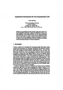
Figure 1. There are many similar “patterns” in the load traces To deal with this kind of error, we predict the load at a possible turning point based on the information of previous similar “patterns”. Our observation of the load traces shows that there are many successive and similar “patterns” occurring in the time series. As shown in Figure 1, such a pattern occurs repeatedly: the time series decreases successively for several times and then one turning point happens, after this turning point the series decreases successively again, and after several times another turning point is reached. We call the successive increases or decreases between two neighboring turning points a “pattern”, and two patterns with same number of data points are thought to be “similar”. Because of this observation, we can predict the value of a possible turning point based on the previous similar pattern: if the point to be predicted comes after several (at least 3) successive decreases (the first point of these successive decreases is a turning point), while the same number of successive decreases can be seen before this series of decreasing points, then we assume that the current point to be predicted is quite possibly a turning point and these two successively decreasing series are two similar “patterns”, so we use the measurement value of the last turning point as the prediction value for the current point, PT+1. If we can’t find such similar pattern we will still use the polynomial fitting method to predict this point. For the prediction of a point following a turning point or two steps after a turning point, a polynomial fitting based prediction will also result in a large error because its prediction involves the use of the turning point, so we predict such points also based on similar patterns: we use the increment for the point after the

previous turning point (or accordingly two steps after last turning point) as the increment for this point. To predict a point after several (at least 3) successive increases, if we can find a successively increasing pattern immediately before this series of increasing points, we use the information of this pattern to judge if current point is a turning point or not and then predict: if the number of points in this pattern has arrived at the same number of the last pattern, then we think that next point will be a turning point and use the measurement of last turning point as PT+1; if the number here is less than that of last pattern, then we use polynomial fitting to predict next value; if we can’t find a successively increasing series we will predict using a “conservative” strategy: we use VT as PT+1. For the other cases we also choose a conservative prediction strategy that sets the increment (decrement) between VT and PT+1 at 0.

deviation is 0.14. The total number of data in this time series is 1,123,200 (for 65 days). sahara.cmcl.cs.cmu.edu is a moderately loaded (mean load 0.22), big memory compute server. The stand deviation of the CPU load is 0.33. The total number of data in this time series is 345,600 (for 20 days). themis.nectar.cs.cmu.edu is a moderately loaded (mean load 0.49) desktop machine. The load on this machine has high standard deviation of 0.5. The total number of data in this time series is 345,600 (for 20 days).

(1) axp0.psc.edu

(2) axp7.psc.edu

4. Experimental evaluations 4.1 Experimental environment We ran a series of experiments using our prediction method to evaluate its effectiveness under load traces with a variety of statistical properties. The load traces we used are the load time series set on a Unix system and were collected by Dinda [16]. The load on a Unix system at any time is the number of processes that are running or ready to run. The kernel samples the number at some period and exponentially averages some previous samples to produce a load average. To satisfy the Nyquist criterion, Dinda chose a 1 HZ sample rate and exponentially averaged with a time constant of five seconds. This captures all of the dynamics made available to us by the operating system. Specifically we evaluated our one-step-ahead time series prediction strategy on CPU load time series collected from four heterogeneous machines. These four machines demonstrate different CPU statistical properties, as illustrated in Figure 2. There are two groups of machines. The first is in an Alpha cluster. Of this group, the machine axp0 is an interactive machine, while axp7 is a batch machine. The machines in the second group are a compute server (sahara) and a desktop workstation (themis). axp0.psc.edu is a heavily loaded, highly variable interactive machine with mean CPU load 1 and stand deviation 0.54. The total number of data in this time series is 1,296,000 (for 75 days). axp7.psc.edu is a more lightly loaded batch machine which has interesting epochal behavior. The average of the CPU load is only 0.12 and its stand

(3)sahara.cmcl.cs.cmu.edu

(d) themis.nectar.cs.cmu.edu

Figure 2. CPU load time series collected from four machines

4.2 Evaluation results for the two strategies The evaluation results, using our prediction strategy to predict the CPU load on these four machines, are shown in Table 1. Here the prediction error for a measurement is the ratio between the absolute value of prediction error (the difference between a predicted value and the measurement) and the measurement. The mean and standard deviation of prediction errors are, respectively, the average error ratio and standard deviation for the prediction error ratios of all the data in a time series. Since it has been proved that the tendency-based prediction strategy outperforms the NWS method, we only conducted a comparison with the tendency-based method, as shown in Table 1. For the data set on each machine we evaluated the two strategies using different numbers of data from 1 day to the total number of the data. Since data exhibits different statistical properties at different times, the prediction error has no direct relationship with the amount of data, but from the experimental results we can see that in all cases our prediction method performs significantly better than the tendency-based method for all of the four load traces

which reveal different load properties. For the time series on axp0 our method predicts 38% to 48% more accurately than the tendency-based strategy. On the sahara compute server our method reduces the average prediction error rate by 40% to 68%, while on the desktop machine themis our method is 37% to 63%

better than the tendency-based method. On the lightly loaded, lowly variable batch machine axp7 our prediction strategy achieves the best prediction error reduction ratio (82% to 86%). Compared with the tendency-based method, our strategy is especially effective for predicting CPU load on machine axp7.

Table 1. The comparison of prediction errors of the two prediction strategies (1) mean and standard deviation of the prediction errors on time series collected from axp0.psc.edu 1day axp0

5days

Mean (%) 10.58

0.43

Our method

6.54

0.20

Reduction ratio

38%

Tendency-based

SD

10days

Mean (%) 13.73

0.54

7.86

0.22

SD

43%

Mean (%) 15.93 8.31

15days

SD 0.4 0.33

48%

Mean (%) 16.32 9.33

20days

0.47

Mean (%) 16.8

0.28

10.14

SD

43%

75 days

0.48

Mean (%) 18.99

0.44

0.39

10.57

0.37

SD

40%

SD

44%

(2) mean and standard deviation of the prediction errors on time series collected from axp7.psc.edu axp7 Tendency-based

1day Mean SD (%) 20.45 0.22

Our method

3.14

Reduction ratio

85%

0.16

5days Mean SD (%) 18.0 0.26 3.06

0.23

83%

10days Mean SD (%) 17.02 0. 39 2.92

0. 13

83%

15days Mean SD (%) 15.34 0.29 2.83

20days Mean SD (%) 20.45 0.32

0.07

2.81

82%

65 days Mean SD (%) 15.02 0.38

0.08

2.73

86%

0.08

82%

(3) mean and standard deviation of the prediction errors on time series collected from sahara.cmcl.cs.cmu.edu sahara

1day

5days

10days

Mean(%)

SD

Mean(%)

SD

Tendency-based

23.59

0.33

20.9

Our method

7.54

0.25

9.86

Reduction ratio

68%

15days

20days

Mean(%)

SD

Mean(%)

SD

Mean(%)

SD

0.35

20.2

0.26

18.74

0.34

18.28

0.37

0.31

10.31

0.12

11.33

0.21

9.2

0.23

53%

49%

40%

50%

(4) mean and standard deviation of the prediction errors on time series collected from themis.nectar.cs.cmu.edu themis

1day

5days

10days

15days

20days

Mean(%)

SD

Mean(%)

SD

Mean(%)

SD

Mean(%)

SD

Mean(%)

SD

3.13

0.05

20.3

0.55

25.85

0.34

27.48

0.51

27.37

0.48

Our method

1.97

0.05

8.93

0.4

9.51

0.04

11.39

0.14

10.6

0.25

Reduction ratio

37%

Tendency-based

56%

5. Conclusion Predictions of future system performance can be used to improve resource selection and scheduling in a dynamic grid environment. In this paper we propose and evaluate a novel one-step-ahead CPU load prediction strategy which conducts the prediction based on the increase or decrease tendency in several past steps and on previous similar patterns, using a polynomial fitting method. The experiment results we conducted demonstrate that this new prediction

63%

59%

61%

strategy outperforms the previously best tendencybased method with average prediction errors that are 37% to 86% lower than those incurred by the tendency-based method.

References [1] I. Foster and C. Kesselman, The Grid: Blueprint for a New Computing Infrastructure, Morgan Kaufmann Publishers, San Fransisco, CA, 1999. [2] P.A. Dinda, D.R. O'Hallaron, “Host load prediction using linear models,” Cluster Computing 3(4), pp. 265-

280, 2000. [3] L. Yang, J.M. Schopf, and I. Foster, “Conservative scheduling: Using predicted variance to improve decisions in dynamic environment,” Supercomputing’03, pp. 1-16, 2003. [4] P.A. Dinda, “A prediction-based real-time scheduling advisor,” Proc. 16th Int’l Parallel and Distributed Processing Symp.(IPDPS 2002), pp. 35-42, 2002. [5] D. Lu, H. Sheng, and P. Dinda, “Size-based scheduling policies with inaccurate scheduling information,” 12th IEEE Int’l Symp. on Modeling, Analysis, and Simulation of Computer and Telecommunications Systems(MASCOTS'04), pp. 31-38, 2004. [6] S. Jang, X. Wu, and V. Taylor, “Using performance prediction to allocate grid resources,” Technical report, GriPhyN 2004-25, pp. 1-11, 2004. [7] L. Yang, I. Foster, and J.M. Schopf, “Homeostatic and tendency-based CPU load predictions,” Int’l Parallel and Distributed Processing Symp. (IPDPS'03), pp. 42-50, 2003. [8] R. Wolski, N. Spring, and J. Hayes, “Predicting the CPU Availability of Time-shared Unix Systems on the Computational Grid,” Proc. 8th IEEE Symp. on High Performance Distributed Computing, pp. 1-8, 1999. [9] M. Swany and R. Wolski, “Multivariate resource performance forecasting in the network weather service,” Supercomputing’02, pp. 1-10, 2002. [10] R. Wolski, “Dynamically forecasting network performance using the network weather service,” Journal of Cluster Computing, Vol.1, pp.119-132, 1998. [11] R. Wolski, “Experiences with predicting resource performance on-line in computational grid settings,” ACM SIGMETRICS Performance Evaluation Review, Vol.30, No.4, pp. 41-49, 2003. [12] P.A. Dinda, “The statistical properties of host load,” Technical report, CMU, pp. 1-23, 1998. [13] S. Akioka and Y. Muraoka, “Extended forecast of CPU and network load on computational grid,” 2004 IEEE Int’l Symp. on Cluster Computing and the Grid, pp. 765-772, 2004. [14] J. Liang, K. Nahrstedt, and Y. Zhou, “Adaptive MultiResource Prediction in Distributed Resource Sharing Environment,” 2004 IEEE Int’l Symp. on Cluster Computing and the Grid, pp. 1-8, 2004. [15] G. Box, G. Jenkins, and G. Reinsel, Time Series Analysis, Forecasting and Control, Prentice Hall, 1994. [16] http://www.cs.cmu.edu/~pdinda/LoadTraces/