in Pentium architecture. Benchmarks as FPU Winmark ([3]), working with floating numbers, showed that Pentium 4 is particularly slow compared to Pentium 3.
A Java CPU calibration tool for load balancing in distributed applications Guilhem Paroux, Bernard Toursel, Richard Olejnik, Violeta Felea University of sciences and technologies of Lille Laboratoire d’Informatique Fondamentale de Lille (UMR CNRS 8022) 59655 Villeneuve d’Ascq Cedex FRANCE Email: (paroux; toursel; olejnik; felea)@lifl.fr
Abstract— This article presents a method for evaluating the CPU powers, independently from the system used, in heterogeneous network of workstations context. It is based on the use of Java language in order to ensure application portability and more particularly on the mechanism of thread CPU processing time measurement introduced into the version 1.5 of Sun Java. That tool will be integrated into the load balancing mechanism which is totally written in Java and that we developed in LIFL project ADAJ. We show how to evaluate the potential power of the CPU with a software totally written in Java. Moreover, we will justify the results provided by our approach. We will also replace the calibration tool in the contexts of distributed applications and of load balancing in a network of workstations.
I. K EYWORDS Calibration, Java, CPU time, Network of workstations, Distributed systems, Load observation II. I NTRODUCTION Usual networks of workstations, such as clusters, large distributed systems or grids, are very often composed of heterogeneous hardwares and systems (in this paper, we will always use the abbreviation NOW to speak about network of workstation). The heterogeneity poses problems about the deployment and the load balancing of distributed applications. It is not efficient to give more work to a station not very workloaded but which is slow. Calculations will be done slowly and the high delivery period of results will delay new tasks beginning or make some tasks idle, waiting for these results. The purpose of the tool presented in this paper is to allow a classification of the stations composing a NOW according to their speed. The result will be taken into account at the load balancing time as well as the load measurement. The combination of these two factors, load and CPU power, will enable to consider the promising character of a node following its capacity to quickly carry out its allocated tasks. We will describe first the context in which calibration takes place : ADAJ environment and the tool utility. Then we will present the concepts that we have implemented in our tool. We continue by studying the results provided by calibration. Finally, we will see the use of the results in load balancing.
III. G ENERAL CONTEXT High performance calculation lies more and more on heterogeneous NOWs which have low cost and are more available than massively parallel machines. But the station heterogeneity and availability pose new problems when distributing the works between the NOW nodes. It is necessary to consider the power differences between the stations as an additional constraint. It is indeed not desirable to entrust the same quantity of work to two stations similarly workloaded but having distinct computing powers. For that, it is necessary to know how to evaluate the potential computing power of NOW nodes and to take it into account at the work distribution time. Traditionally, the load balancing is carried out in two phases. The first consists in measuring the node loads then to classify those in several categories : underloaded, normally loaded and overloaded. In case of an unbalanced situation, the second phase determines which are the objects to be migrated and what could be their new hosts. In our case, the measurement of load must be balanced by the CPU computing power in order to take into account the variable delivery period of the results between workstations. The global project in which takes place the work presented in that paper is ADAJ project (Adaptative Distributed Application in Java). ADAJ ([4], [5], [9], [11], [12], [6]) gives a distribution and execution environment for distributed applications. It provides also the tools necessary to the distribution of the objects in the NOW as well as a system of load balancing. It is written in Java language in order to keep compatibility on many platforms. It is based more specifically on RMI, the Java ([1]) remote object call system, and on Javaparty ([2]) to manage the distribution and execution environment of the distributed applications. A load balancing mechanism has been implanted in the ADAJ platform. This mechanism is based on a new observation tool, written in Java, which measures the activities (computing and communication) of objects into the JVM. However, it considers only intra-application load balancing without taking into consideration the workstation load external to the JVM. The new objective is to extend the load balancing mechanism of ADAJ by taking into account characteristics which are
external to the applications and to the JVMs. For example, the workstation architecture and the operating system used is not the same in all the NOW. Other applications can use the CPU and we have no way to control them. We have to take into account their CPU processing time and to react in our application. As we have already said, the workstations have quite different computing powers. This implies that the same work quantity will not be executed in the same time by a powerful workstation and another slower. In order to balance the workload measures, it is necessary to know each workstation computing power. Thus, workload comparison will be done both on the work quantity on the workstation and on its ability to carry out this work in a short time. The tool presented in this paper enables to evaluate workstations computing power and to assign a power rating to each one by comparing the calibration thread result of each workstation. It is what we will develop now. IV. P RESENTATION OF CALIBRATION
TOOL
The goal of calibration is not to provide an accurate measurement of a workstation power by considering all the aspects of the traditional benchmarks : inputs-outputs, CPU, network, etc. It is simply a question of having a quite good approximation of the workstation potential computing power. We will thus be interested primarily in the CPU calculation speed measurement in order to correct the workload evaluated in a station by the power of this station. The operation principle is simple : every workstation receives the same small program to be carried out, consequently the same quantity of work, and returns time spent to carry out all the code. Next, the results are compared together and a classification is done between the workstations. A first approach consists in recovering the machine’s system time once at the execution beginning and in a second time at the end. The difference between the two instantaneous times gives the time spent during the execution. This method requires to take into account the workstation load. Indeed, if the computer is occupied by a lot of processes, competition to reach the CPU will be important and processes will spend apparently more time to be executed. This need to know the station workload (by using specific system functions) in order to evaluate the real computing power. However, this solution is more difficult to be implemented and does not allow portability. Moreover the approximations become too important and the results are not usable. The problem of the execution time variability can easily be avoided. A quantity of work being executed on a given processor receives an almost constant CPU time quantity whatever is the machine workload. This is due to the fact that the program has some elementary instruction sequence to execute which takes a determined time depending on the CPU type and frequency. By measuring time which the thread was allocated the CPU, we do not need to take care about workstation load in our calibration. In order to respect the constraint of portability in a heterogenenous
NOW, the calibration tool is totally designed in Java. A specific calibration thread is executed in every JVM. To recover the time spent on the CPU by our thread, we use a new package of Java (java.lang.management) included in the last version 1.5 of the Sun SDK. We more particularly use the ThreadMBean interface which comprises methods to question the JVM on the threads that are running. The threads identifier, their names, their states and especially their CPU processing times are thus recovered. By calling the method getThreadCpuTime() by our calibration thread, we obtain a good approximation of the observed CPU computing power. Lesser is the processing time, higher is the CPU computing power. We do not obtain an absolute computing power but by comparing the processing times found on every workstations, we can classify them and allot a power rating to each one. The program presents only few interest. Its only goal is to give some works to the CPU and to return its own processing time. However, we want to specify that it manipulates two data types : integers and floating numbers. This choice was made in order to not favour one particular data type on which an architecture could take advantage. For instance some CPU architectures behave better with the integers than with the floating numbers. This fact will be pointed out when we will present the results in the following section.
V. R ESULT PRESENTATION AND
COMMENTS
We should first specified that the Java threads launched in the JVM are treated as native threads and thus recognized as independent processes by the scheduler. During our tests, we used different types of programs to load the workstation. We observed that external processes and internal threads had the same effects on our measures. By another way, we will speak about CPU processing time and total execution time. The first means the time spent using the CPU by a thread while the second means the elapsed time between the beginning and the end of the thread execution. The second is altered by other process execution which access to the CPU. Let us interest now in the results of the tests carried out on several machines which are representative of a heterogeneous NOW by their architecture differences. We carried out a measurement serie on each station by launching the calibration tool 8 times and by varying the machine load. The obtained results show that CPU time allocated by the scheduler to our calibration thread is a function of the workstation computing power and is independant of the effective station workload. On other hand the total execution time of the calibration thread is a function of the load. The used CPUs are as follows : INTEL Pentium 3 600 MHz INTEL Pentium 3 860 MHz INTEL Pentium 4 1500 MHz AMD Athlon 1800+ 1500 MHz INTEL Pentium 4 2600 MHz Hyperthreading Activated INTEL Pentium 4 2800 MHz Hyperthreading Deactivated INTEL Pentium 4 3000 MHz Hyperthreading Activated
TABLE I
We will consider the concept of Hyperthreading at the time of the results analysis in order to better explain it and its effects to our measurements.
CPU PROCESSING TIME
25000 ’P3_600’ ’P3_860’ ’P4_1500’ ’ATHLON_1500’ ’P4_2600_HT’ ’P4_2800_noHT’ ’P4_3000_HT’
CPU time for our thread in milliseconds
20000
Processor
Integer
Float
Pentium 3 860
9000 ms
7200 ms
Pentium 4 1500
7000 ms
7900 ms
Let us see now the second curve serie that shows the calibration thread total execution time in order to carry out all its instructions. These curves will enable us to propose the quality of the previous results by noticing that they well reflect the real CPU performance.
15000
10000
’P3_600’ ’P3_860’ ’P4_1500’ ’ATHLON_1500’ ’P4_2600_HT’ ’P4_2800_noHT’ ’P4_3000_HT’
1.2e+06
Elapsed time to calculate our thread in milliseconds
5000
0 0
Fig. 1.
5
10
15
20 25 30 Number of running processes
35
40
45
50
CPU processing time for different CPUs
The curve serie presented in Fig.1 illustrates the constancy of CPU time which are allocated to the calibration thread while the machine load is increasing. This time is constant on a given machine and is linked with the CPU performance. The constancy is due to the fact that the instruction sequence takes always the same time to be executed. Concerning the differences between the measured running time of CPUs, we note that times are not directly connected with the CPU frequency. This is normal because it is known that a double frequency processor is not twice faster. Performance improvement results both from technological and architecture progresses. We will see later that the processing time found must be balanced with the number of processors. Thus the differences between the execution times found on Pentium 3 600 MHz and Pentium 3 860 MHz are important (approximately 23100 ms compared to 16200 ms) for only 260 MHz of difference between frequencies. In addition, the differences in execution time between Pentium 3 860 MHz and Pentium 4 1500 MHz are very reduced (16200 ms on a side and 14900 ms of the other) in spite of a strong difference on the frequency level. This results mainly from the differences in Pentium architecture. Benchmarks as FPU Winmark ([3]), working with floating numbers, showed that Pentium 4 is particularly slow compared to Pentium 3. On the other hand, Pentium 4 is faster for calculation of integers than Pentium 3. Benchmark CPU Mark 99 ([3]), working with integers, shows this fact. Our thread deals with the two data types for calculations in order to show that for current use(mixing integers and floating numbers), the results are favorable to Pentium 4. We deliver however the intermediate results of integer and floating numbers calculation in order to point out the Pentium 4 slower execution with floating numbers. This justifies the use of both floating numbers and integers.
1e+06
800000
600000
400000
200000
0 0
Fig. 2.
5
10
15
20 25 30 Number of running processes
35
40
45
50
Total execution time evolution with workload
The results presented in Fig.2 are in accordance with the forecasts : the real execution time increases with the process number. Our thread receives less and less CPU time when the CPU is required by a growing number of processes. An interesting result is that the speed ratio between two CPU types is constant whatever is the workload. Moreover, we observe a coherence of the two measure types. Let us take some values to illustrate this matter with Pentium 3 600 MHz versus Pentium 3 860 MHz. TABLE II R ATIO BETWEEN TWO CPU S Processor
Processing
5 threads
20 threads
50 threads
P3 600
23100 ms
139085 ms
487598 ms
1188254 ms
P3 860
16200 ms
96780 ms
336995 ms
825603 ms
Ratio
1.426
1.437
1.447
1.439
The first computing power ratio (1.426) found thanks to CPU processing time measurement is confirmed by measurements which reflect the time really taken by the thread to deliver these results. That shows that the first measurement is good and sufficient to classify the workstations according to
their computing power. Let us interest in another figure serie in which was used the last Pentium 4 where Hyperthreading was activated. Let us observe the behavior of Pentium 4 1500 MHz compared to Pentium 4 2600 MHz using Hyperthreading: TABLE III R ATIO BETWEEN TWO CPU S Processor
Processing
5 threads
20 threads
50 threads
P4 1500
14900 ms
90622 ms
313552 ms
765540 ms
P4 2600
12000 ms
36614 ms
134383 ms
312447 ms
Ratio
1.242
2.475
2.333
2.450
The ratios found by comparing the real execution times are very close but do not correspond to the ratio found in CPU processing time measurements. The values are on the other hand very close to twice the initial value. An explanation is to be found in Hyperthreading technology. This process developped by INTEL makes it possible to simulate the operation of a bi-processor with only one Pentium 4. The physical processor is in fact built with two logical processors which are able to carry out each one a calculation by clock cycle, the processor computing power is thus doubled on the level of the physical processor. The results found in the case of the real execution time must be linked with the fact that on a traditional processor the processes are carried out one by one in competition while with Hyperthreading they are carried out two by two. This assertion is confirmed by the results that we obtained with real time : Pentium 4 1500 MHz with 10 threads : 165833 ms Pentium 4 2600 MHz Hyperthreading with 20 threads : 134383 ms The ratio is 1.234 which corresponds to the ratio of computing power initially found. The comparison between the two processors is possible by taking into account the double of processes on that managing Hyperthreading. This behaviour is expected since the processor simulates the operation of two processors in parallel. When the measure takes into account just one running process on a multi-processor system, the advantage is not real. On the contrary, when several processes are running, the processes are dispatched on the different processors, so they are executed faster. In this case, our measurement, which is a function of the global load, shows the different behaviours. This remark enables us to conclude on the fact that the workstation calibration must also take into account the number of processors present on the machine. That leads us to consider the results obtained with Pentium 4 2800 MHz when Hyperthreading is deactivated. The CPU processing time for calibration is lower in this case than those for Pentium 4 3000 MHz and 2600 MHz with Hyperthreading activated. This unexpected observation have to be linked with the fact that in measurements of total execution time, the following results are found : the processor without Hyperthreading is slower. This surprising result explanation holds
in the Hyperthreading operation. The physical processor is single even if it simulates two logical processors and thus the level-2 cache is alone and must manage the competitor accesses between the two logical processors. When we are interested in the real computing time, the latencies to reach the memory are masked by the profit of execution speed due to the presence of the two logical processors. By observing the behavior at the level of only one thread, latencies are quite visible. This explains the fact that lower computing time are found on the processor whose Hyperthreading was deactivated. On the other hand it should be noticed that in the case of the total execution time measurement, the relationship between the various processors values remains constant whatever the workstation load; the results are thus valid. We have just seen that the results provided by the tool for calibration reflect the workstation power. The cases of Hyperthreading and the multiprocessors systems are automatically taken into account by recovering the number of processors thanks to the Java function java.lang.Runtime.availableProcessors() and by taking into account this number in the use of the results, which we will see now. VI. C ALIBRATION
USE
The calibration tool returns two items of information for each station : the CPU processing time for the execution of a given thread and the available processor number. As we consider network of workstations, the calibration interest is to be able to classify the nodes according to their potential computing power. The first classification considered consists in separating the stations in 3 categories : fast, average, slow. This method makes it possible to have a simple classification of the NOW nodes. The computer pool will influence the load migration decisions which are to take thereafter in order to balance the machine load measured by the tool we have developed. Thus for instance, a powerful and loaded station will be privileged compared to another very slow but not very loaded. This is done in spite of an apparent difference in workload which should have played in favour of the second. However, this way of classifying the stations has several disadvantages. Firstly, it does not allow a fine distinction between machines of different computing powers which are classified in the same category. Secondly, the statistical tools used (average, standard deviation) lead to advantage the average category and disavantage the extreme cases. Lastly, the addition of a new station is followed by a new workstations classification. All these criticisms do not make it possible to keep this classification. The adopted method provides a power index to each station taking into account its CPU processing time for the calibration thread and the available processor number. Taking into account the processor number is done quite simply by dividing the CPU processing time found by the number of processors. This calculation can appear inaccurate since two processors do not give a station twice more powerful than one using
only one processor. However, the power index that we wish does not need to have an extreme precision and moreover, the results obtained by employing this method are completely satisfactory. Let us have a look on some processor CPU processing time and total execution times (increasing with the workload) measured with 15 processes on the workstation (HT means Hyperthreading). TABLE IV CPU TIME ALLOCATION Processor
Processing
(1)P4 2600 MHz HT
12100 ms
95000 ms
(2)P4 2800 MHz
7800 ms
125000 ms
(3)P4 3000 MHz HT
10000 ms
75000 ms
obtain the load rating which will be used to classify the workstations in the three categories : underloaded, normally loaded, overloaded. The next step is the load balancing phase. Every overloaded workstation choose an object to move depending on the information delivered by the object activity monitor present in the ADAJ environment. This tool observes the number of object instance calls and provides information about object activities and communications. The object migration can now be done and an other cycle begins. VII. C ONCLUSION
Execution (15 threads)
Between (1) and (2) the ratio of CPU allocation times is 1.551 in favour of (2). The real times prior to deliver the results present a ratio of about 1.316 in favour of (1) this time. However, if we divide by 2 the CPU processing time of (1), we obtain a relationship between (1) and (2) of order 1.289 in favour of (1) this time what is in conformity with the ratio found for the real execution time. Between (2) and (3), the conclusions are similar : an apparent ratio of 1.282 favorable to (2) for CPU processing times but a ratio of 1.667 in the real times favorable to (3). While dividing by 2 the time of CPU allocation of (3), we obtain a ratio of 1.560 favorable to (3) that is in conformity with the relationship between the real execution times. Once balanced by the number of processors which can be obtained by a Java method, measurements are usable to provide a power index for each workstation. The lowest indices are assigned to the least powerful workstation and the highest indices to the more powerful stations. These indices will be used in NOW load measurements in order to determine what work migrations are to be operated. During the NOW working, workload measurements are carried out regularly by another tool which cannot be described in this short paper. The results obtained are the percentage of CPU used by the JVM and the running threads amount. As we have already seen, the same quantity of work is not executed similarly by a powerful workstation and by a slower one. For example, the results show that a Pentium 4 2600 MHz HT is more than twice faster than a Pentium 4 1500 MHz. Thus, the Pentium 4 2600 MHz HT can carry out twice more work than the Pentium 4 1500 MHz in the same time. The Fig.2 illustrates very well this assertion. The tool is being integrated in ADAJ. The new version works as follows. First, the calibration tool is running and a power rating is alloted to each workstation. After that, the workload measurement tool delivers results regularly. For a new set of measures, a workload rating is calculated for each workstation. This rating is obtained by multiplicating the power rating and the percentage of CPU time used by one thread in the JVM during a determined time. Thus, we
In order to adapt the measuring instruments for load balancing developed in ADAJ to the case of heterogeneous NOWs, we need to know the potential workstation computing power. It is indeed impossible to compare directly two stations which have different powers and to draw any conclusions. The preliminary workstations calibration makes it possible to differenciate their power. The tool presented in this article is appropriate for this task. It is developed entirely in Java to ensure portability on heterogeneous networks of workstations and we have shown that it is sufficiently accurate for our needs. The CPU processing time is a satisfactory measurement to determine the potential of calculation speed which the station will be able to deliver. Other benchmarks could be use for specific needs, but the CPU calculation speed is sufficiently general to ensure a good evaluation in most of the cases. The tool for calibration will be coupled soon with the mechanism of load measurement currently developed in this same context of heterogeneous NOWs. It will make it possible to refine measurements and to balance the results by holding account of the worstation potential work power and its entrusted work completion speed. R EFERENCES [1] [2] [3] [4]
http://java.sun.com Java Home. http://www.ipd.uka.de/JavaParty/ JavaParty. http://www.hardware.fr/articles/283/page7.html Processor benchmarks. Bouchi A., Olejnik R. and Toursel B.; Java tools for measurement of the machine loads, In Advanced Environments, Tools and Applications for Cluster Computing, Mangalia, Romania, 2001, LNCS 2326, pp. 271-278. [5] Bouchi A., Toursel B. and Olejnik R.; An observation mechanism of distributed objects in Java, 10th Euromicro Workshop on Parallel Distributed and Network-Based Processing, Las Palmas de Gran Canaria, Spain, January 2002. [6] Bouchi A., Olejnik R. and Toursel B.; A new estimation method for distributed Java object activity, 16th IEEE International Parallel and Distributed Processing Symposium, Marriott Marina, Fort Lauderdale, Florida, April 2002. [7] Dahm M.; Byte Code Engineering, JIT’99: Java-Informations-Tage, 1999. [8] Felea V., Devesa N., Lecouffe P. and Toursel B.; Expressing Parallelism in Java Applications Distributed on Clusters, IWCC: NATO International Workshop on Cluster Computing, Romania, September 2001. [9] Felea V. and Toursel B.; Methodology for Java distributed and parallel programming using distributed collections, 16th International Parallel and Distributed Processing Symposium, Marriott Marina, Fort Lauderdale, Florida, April 2002. [10] Felea V.; Exploiting runtime information in load balancing strategy, DAPSYS: Fourth Austrian-Hungarian Workshop on Distributed and Parallel Systems. Linz, Austria, September 2002.
[11] Olejnik R., Bouchi A. and Toursel B.; A Java object policy for load balancing, PDPTA: The international Conference on Parallel and Distributed Processing Techniques and Applications, 2, June 2002, pp. 816-821, Las Vegas, USA. [12] Olejnik R., Bouchi A. and Toursel B.; Object observation for a Java adaptative distributed application platform, PARELEC: International Conference on Parallel Computing in Computing in Electrical Engineering, September 2002, Poland, pp. 171-176. [13] Olejnik R., Bouchi A. and Toursel B.;Observation Policy in ADAJ. Accepted to Parallel and Distributed Computing and Systems (PDCS), USA, 2003. [14] Felea V. and Toursel B.; Middleware-based Load Balancing for Communicating Java Objects, in CIPC Proceedings, Sinaia, Romania, 2003, pp. 177-185. bibitem diffusion Talbi E. - Dynamic allocation of process in the distributed and parallel systems. State of the art, Laboratoire d’Informatique Fondamentale de Lille. report 162. January 1995.