Credit Card Fraud Detection Using Meta-Learning: Issues and Initial Results1 Salvatore J. Stolfo, David W. Fan, Wenke Lee and Andreas L. Prodromidis Department of Computer Science Columbia University 500 West 120th Street New York, NY 10027 {sal,wfan,wenke,andreas}@cs.columbia.edu Philip K. Chan Computer Science Florida Institute of Technology Melbourne, FL 32901
[email protected] Abstract In this paper we describe initial experiments using meta-learning techniques to learn models of fraudulent credit card transactions. Our collaborators, some of the nation’s largest banks, have provided us with real-world credit card transaction data from which models may be computed to distinguish fraudulent transactions from legitimate ones, a problem growing in importance. Our experiments reported here are the first step towards a better understanding of the advantages and limitations of current meta-learning strategies. We argue that, for the fraud detection domain, fraud catching rate (True Positive rate) and false alarm rate (False Positive rate) are better metrics than the overall accuracy when evaluating the learned fraud classifiers. We show that given a skewed distribution in the original data, artificially more balanced training data leads to better classifiers. We demonstrate how meta-learning can be used to combine different classifiers (from different learning algorithms) and maintain, and in some cases, improve the performance of the best classifier. Keywords machine learning, meta-learning, fraud detection, skewed distribution, accuracy evaluation
1
This research is supported in part by grants from DARPA (F30602-96-1-0311), NSF (IRI-96-32225 and CDA-96-25374), and NYSSTF (423115-445).
Introduction A secured and trusted inter-banking network for electronic commerce requires high speed verification and authentication mechanisms that allow legitimate users easy access to conduct their business, while thwarting fraudulent transaction attempts by others. Fraudulent electronic transactions are already a significant problem, one that will grow in importance as the number of access points in the nation’s financial information system grows. Financial institutions today typically develop custom fraud detection systems targeted to their own asset bases. Most of these systems employ some machine learning and statistical analysis algorithms to produce pattern-directed inference systems using models of anomalous or errant transaction behaviors to forewarn of impending threats. These algorithms require analysis of large and inherently distributed databases of information about transaction behaviors to produce models of “probably fraudulent” transactions. Recently banks have come to realize that a unified, global approach is required, involving the periodic sharing with each other information about attacks. Such information sharing is the basis of building a global fraud detection infrastructure where local detection systems propagate attack information to each other, thus preventing intruders from disabling the global financial network. The key difficulties in building such a system are: 1. Financial companies don't share their data for a number of (competitive and legal) reasons. 2. The databases that companies maintain on transaction behavior are huge and growing rapidly, which demand scalable machine learning systems. 3. Real-time analysis is highly desirable to update models when new events are detected. 4. Easy distribution of models in a networked environment is essential to maintain up to date detection capability. We have proposed a novel system to address these issues. Our system has two key component technologies: local fraud detection agents that learn how to detect fraud and provide intrusion detection services within a single corporate information system, and a secure, integrated meta-learning system that combines the collective knowledge acquired by individual local agents. Once derived local classifier agents (models, or base classifiers) are produced at some site(s), two or more such agents may be composed into a new classifier agent (a meta-classifier) by a meta-learning agent. Meta-learning (Chan & Stolfo 1993) is a general strategy that provides the means of learning how to combine and integrate a number of separately learned classifiers or models; a meta-classifier is thus trained on the correlation of the predictions of the base classifiers. The meta-learning system proposed will allow financial institutions to share their models of fraudulent transactions by exchanging classifier agents in a secured agent infrastructure. But they will not need to disclose their proprietary data. In this way their competitive and legal restrictions can be met, but they can still share information. We are undertaking an ambitious project to develop JAM (Java Agents for Meta-learning) (Stolfo et al. 1997), a framework to support meta-learning, and apply it to fraud detection in widely distributed financial information systems. Our collaborators, several major U.S. banks, have provided for our use credit card transaction data so that we can set up a simulated global financial network and study how meta-learning can facilitate collaborative fraud detection. The experiments described in this paper focus on local fraud detection (on data from one bank), with the aim to produce the best possible (local) classifiers. Intuitively, better local classifiers will lead to better global (meta) classifiers. Therefore these experiments are the important first step towards building a high-quality global fraud detection system.
1
Indeed, the experiments helped us understand that fraud catching rate and false alarm rate are the more important evaluation criteria for fraud classifiers, and that training data with more balanced class distribution can lead to better classifiers than a skewed data distribution. We demonstrate that (local) meta-learning can be used to combine different (base) classifiers from different learning algorithms and generate a (meta) classifier that has better performance than any of its constituents. We also discovered some limitations of the current meta-learning strategies, for example, the lack of effective metrics to guide the selection of base classifiers that will produce the best meta-classifier. Although we did not fully utilize JAM to conduct the experiments reported here, due to its current limitations, the techniques and modules are presently being incorporated within the system. The current version of JAM can be downloaded from our project home page: www.cs.columbia.edu/~sal/JAM/PROJECT. Some of the modules available for our local use unfortunately can not be downloaded (e.g., RIPPER must be acquired directly from its owner). Credit Card Transaction Data We have obtained a large database, 500,000 records, of credit card transactions from one of the members of the Financial Services Technology Consortium (FSTC, URL: www.fstc.org). Each record has 30 fields and a total of 137 bytes (thus the sample database requires about 69 mega-bytes of memory). Under the terms of our nondisclosure agreement, we can not reveal the details of the database schema, nor the contents of the data. But it suffices to know that it is a common schema used by a number of different banks, and it contains information that the banks deem important for identifying fraudulent transactions. The data given to us was already labeled by the banks as fraud or non-fraud. Among the 500,000 records, 20% are fraud transactions. The data were sampled from a 12-month period, but does not reflect the true fraud rate (a closely guarded industry secret). In other words, the number of records for each month varies, and the fraud percentages for each month are different from the actual real-world distribution. Our task is to compute a classifier that predicts whether a transaction is fraud or non-fraud. As for many other data mining tasks, we need to consider the following issues in our experiments: Data Conditioning
- First, do we use the original data schema as is or do we condition (pre-process) the data, e.g., calculate aggregate statistics or discretize certain fields? In our experiments, we removed several redundant fields from the original data schema. This helped to reduce the data size, thus speeding up the learning programs and making the learned patterns more concise. We have compared the results of learning on the conditioned data versus the original data, and saw no loss in accuracy. - Second, since the data has a skewed class distribution (20% fraud and 80% non-fraud), can we train on data that has (artificially) higher fraud rate and still compute accurate fraud patterns? And what is the optimal fraud rate in the training data? Our experiments have shown that the training data with a 50% fraud distribution produced the best classifiers. Data Sampling
What percentage of the total available data do we use for our learning task? Most of the machine learning algorithms require the entire training data be loaded into the main memory. Since our database is very large, this is not practical. More importantly, we wanted to demonstrate that metalearning can be used to scale up learning algorithms while maintaining the overall accuracy. In our
2
experiments, only a portion of the original database was used for learning (details provided in the next section). Validation/Testing
How do we validate and test our fraud patterns? In other words, what data samples do we use for validation and testing? In our experiment, the training data were sampled from earlier months, the validation data (for meta-learning) and the testing data were sampled from later months. The intuition behind this scheme is that we need to simulate the real world environment where models will be learned using data from the previous months, and used to classify data of the current month. Accuracy Evaluation
How do we evaluate the classifiers? The overall accuracy is important, but for our skewed data, a dummy algorithm can always classify every transaction as non-fraud and still achieves 80% overall accuracy. For the fraud detection domain, the fraud catching rate and the false alarm rate are the critical metrics. A low fraud catching rate means that a large number of fraudulent transactions will go through our detection system, thus costing the banks a lot of money (and the cost will eventually be passed to the consumers!). On the other hand, a high false alarm rate means that a large number of legitimate transactions will be blocked by our detection system, and human intervention is required in authorizing such transactions (thus frustrating too many customers, while also adding operational costs). Ideally, a cost function that takes into account both the True and False Positive rates should be used to compare the classifiers. Because of the lack of cost information from the banks, we rank our classifiers using first the fraud catching rate and then (within the same fraud catching rate) the false alarm rate. Implicitly, we consider fraud catching rate as much more important than false alarm rate. Base Classifiers Selection Metrics
Many classifiers can be generated as a result of using different algorithms and training data sets. These classifiers are all candidates to be base classifiers for meta-learning. Integrating all of them incurs a high overhead and makes the final classifier very complex (i.e., less comprehensible). Selecting a few classifiers to be integrated would reduce the overhead and complexity, but potentially decrease the overall accuracy. Before we examine the tradeoff, we first examine how we select a few classifiers for integration. In addition to True Positive and False Positive rates, the following evaluation metrics are used in our experiments: 1. Diversity (Chan 1996): using entropy, it measures how differently the classifiers predict on the same instances 2. Coverage (Brodley and Lane 1996): it measures the fraction of instances for which at least one of the classifiers produces the correct prediction. 3. Correlated Error (Ali and Pazzani 1996): it measures the fraction of instances for which a pair of base classifiers makes the same incorrect prediction. 4. Score: 0.5 * True Positive Rate + 0.5 * Diversity This simple measure approximates the effects of bias and variance among classifiers, and is purely a heuristic choice for our experiments. Experiments To consider all these issues, the questions we pose are:
3
• • •
What is the best distribution of frauds and non-frauds that will lead to the best fraud catching and false alarm rate? What are the best learning algorithms for this task? ID3 (Quinlan 1986), CART (Breiman et al.1984), RIPPER (Cohen 1995), and BAYES (Clark and Niblett 1987) are the competitors here. What is the best meta-learning strategy and best meta-learner if used at all? What constitute the best base classifiers?
Other questions ultimately need to be answered: • How many months of data should be used for training? • What kind of data should be used for meta-learning validation? Due to limited time and computer resources, we chose a specific answer to the last 2 issues. We use the data in month 1 through 10 for training, and the data in month 11 is used for meta-learning validation. Intuitively, the data in the 11th month should closely reflect the fraud pattern in the 12th month and hence be good at showing the correlation of the predictions of the base classifiers. Data in the 12th month is used for testing. We next describe the experimental set-up. •
Data of a full year are partitioned according to months 1 to 12. Data from months 1 to 10 are used for training, data in month 11 is for validation in meta-learning and data in month 12 is used for testing.
•
The same percentage of data is randomly chosen from months 1 to 10 for a total of 42000 records for training.
•
A randomly chosen 4000 data records from month 11 are used for meta-learning validation and a random sample of 4000 records from month 12 is chosen for testing against all learning algorithms.
•
The 42000 record training data is partitioned into 5 parts of equal size: f: pure fraud nf1 , nf3 , nf3 , nf4 : pure non-fraud
•
The following distribution and partitions are formed: 1. 50%/50% frauds/non-frauds in training data: 4 partitions by concatenating f with one of nfi 2. 33.33% /66.67%: 3 partitions by concatenating f with 2 randomly chosen nfi 3. 25%/75%: 2 partitions by concatenating f with 3 randomly chosen nfi 4. 20% /80%: the original 42000 records sample data set
4
•
4 Learning Algorithms: ID3, CART, BAYES, and RIPPER. Each is applied to every partition above. We obtained ID3 and CART as part of the IND (Buntime 1991) package from NASA Ames Research Center. Both algorithms learn decision trees. BAYES is a Bayesian learner that computes conditional probabilities. BAYES was re-implemented in C. We obtained RIPPER, a rule learner, from William Cohen.
•
Select the best classifiers for meta-learning using the class-combiner (Chan & Stolfo 1993) strategy according to the following different evaluation metrics: Classifiers with the highest True Positive rate (or fraud catching rate); Classifiers with the highest diversity rate; Classifiers with the highest coverage rate; Classifiers with the least correlated error rate; Classifiers with the highest Score.
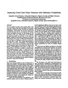
The experiments were run twice and the results we report next are computed averages. Including each of the combinations above, we ran the learning and testing process for a total of 1,600 times. Including accuracy, True Positive rate and False Positive rate, we generated a total of 4800 results. Results Of the results generated for 1600 runs, we only show True Positive and False Positive rate of the 6 best classifiers in Table 1. Detailed information on each test can be found at the project home page at: www.cs.columbia.edu/~sal/JAM/PROJECT. There are several ways to look at these results. First, we compare the True Positive rate and False Positive rate of each learned classifier. The desired classifier should have high fraud catching (True Positive) rate and relatively low false alarm (False Positive) rate. The best classifier among all generated is a meta-classifier: BAYES used as the meta-learner combining the 4 base classifiers with the highest True Positive rates (each trained on a 50%/50% fraud/non-fraud distribution). The next two best classifiers are base classifiers: CART and RIPPER each trained on a 50%/50% fraud/non-fraud distribution. These three classifiers each attained a True Positive rate of approximately 80% and False Positive rate less than 17% (with the meta-classifier begin the lowest in this case with 13%). To determine the best fraud distribution in training data for the learning tasks, we next consider the rate of change of the True Positive/False Positive rates of the various classifiers computed over training sets with increasing proportions of fraud labeled data. Figures 1 and 2 display the average True Positive/False Positive rates for each of the base classifiers computed by each learning program. We also display in these figures the True Positive/False Positive rates of the meta-classifiers these programs generate when combining base classifiers with the highest True Positive rates. Notice the general trend in the plots suggesting that the True Positive and False Positive rates increase as the proportion of fraud labeled data in the training set increases. When the fraud distribution goes from 20% to 50%, for both CART and RIPPER, the True Positive rate jumps from below 50% to nearly 80%. In this experiment, 50%/50% is the best distribution with the highest fraud catching rate and false alarm rate. We also notice that there is an increase of false alarm rate from 0% to slightly more than 20% when the fraud distribution goes from 20% to 50%. (We have not yet completed a full round of experiments on higher
5
proportions of fraud labeled data. Some preliminary results we have show that the True Positive rate only slightly degrades when fraud labeled data dominates in the training data set, but the False Positive rate increases rapidly. The final version of the paper will detail these results, which are not entirely available at the time of submissions.) Notice that the best base classifiers were generated by RIPPER and CART. As we see from the results (partially shown in Table 1) across different training partitions and different fraud distributions, RIPPER and CART have the highest True Positive rate (80%) and reasonable False Positive rate (16%) and their results are comparable to each other. ID3 performs moderately well, but BAYES is remarkably worse than the rest, it nearly classifies every transaction to be non-fraud. This negative outcome appears stable and consistent over each of the different training data distribution. As we see from Figure 4 and Table 1, the best meta-classifier was generated by BAYES under all of the different selection metrics. BAYES consistently displays the best True Positive rate, comparable to RIPPER and CART when computing base classifiers. However, the meta-classifier BAYES generates displays the lowest False Positive rate of all. It is interesting to determine how the different classifier selection criteria behave when used to generate meta-classifiers. Figure 4 displays a clear trend. The best strategy for this task appears to be to combine base classifiers with the highest True Positive rate. None of the other selection criteria appear to perform as well as this simple heuristic (except for the least correlated errors strategy which performs moderately well). This trend holds true over each of the training distributions. Table 1 Results of Best Classifiers Classifier Name BAYES as meta-learner combining 4 classifiers (earned over 50%/50% distribution data) with highest True Positive rate RIPPER trained over 50%/50% distribution CART trained over 50%/50% distribution BAYES as meta-learner combining 3 base classifiers (trained over 50%/50% distribution) with the least correlated errors BAYES as meta-learner combining 4 classifiers learned over 50%/50% distribution with least correlated error rate ID3 trained over 50%/50% distribution
True Positive (or Fraud Catching Rate)
False Positive (or False Alarm Rate)
80%
13%
80%
16%
80%
16%
80%
19%
76%
13%
74%
23%
6
In one set of experiments, based on the classifier selection metrics described previously, we pick the best 3 classifiers from a number of classifiers generated from different learning algorithms and data subsets with the same class distribution. In Figure 3, we plotted the values of the best 3 classifiers for each metric against the different percentages of fraud training examples. We observe that both the average True Positive rate and the average False Positive rate of the three classifiers increase when the fraction of fraud training examples increases. We also observe that diversity, hence score, increases with the percentage. In a paper by two of the authors (Chan and Stolfo, 1997), it is noted that base classifiers with higher accuracy and higher diversity tend to yield meta-classifiers with larger improvements in overall accuracy. This suggests that a larger percentage of fraud labeled data in the training sets will improve accuracy here. Notice that coverage increases and correlated error decreases with increasing proportions of fraud labeled training data. However, the rate of change (slope) is much smaller than the other metrics. Discussion and Future Work The result of using 50%/50% fraud/non-fraud distribution in training data is not coincident. Other researchers have conducted experiments with 50%/50% distribution to solve the skewed distribution problem on other data sets and have also obtained good results. We have confirmed that 50%/50% improves the accuracy for the all the learners under study. The experiments reported here were conducted twice on a fixed training data set and one test set. It will be important to see how the approach works in a temporal setting: using training data and testing data of different eras. For example, we may use a “sliding window” to select training data in previous months and predict on data of the next one month, skipping the oldest month in the sliding window and importing the new month for testing. These experiments also mark the first time that we apply meta-learning strategies on real-world problems. The initial results are encouraging. We show that combining classifiers computed by different machine learning algorithms produces a meta-classification hierarchy that has the best overall performance. However, we as yet are not sure of the best selection metrics for deciding which base classifiers should be used for meta-learning in order to generate the best meta-classifier. This is certainly a very crucial item of future work.
Conclusion Our experiments tested several machine learning algorithms as well as meta-learning strategies on realworld data. Unlike many reported experiments on “standard” data sets, the set up and the evaluation criteria of our experiments in this domain attempt to reflect the real-world context and its resultant challenges. The KDD process is inherently iterative (Fayyad et al. 1996). Indeed, we have gone through several iterations of data conditioning, sampling, mining (applying machine learning algorithms on) the data, and evaluating the patterns. We then came to realize that the skewed class distribution could be a major factor on classifier performance and that True and False Positive rates are the critical evaluation metrics. We conjecture that, in general, the exploratory phase of the data mining process can be helped in part, for example, by purposely applying different families of stable machine learning algorithms to the data and comparing the classifiers. We may then be able to deduce the “characteristics” of the data, which can help us choose the most suitable machine learning algorithms and meta-learning strategy.
7
The experiments reported here indicate: 50%/50% distribution of fraud/non-fraud training data will generate classifiers with the highest True Positive rate and low False Positive rate so far. Other researchers also reported similar findings. Meta-learning with BAYES as a meta-learner to combine base classifiers with the highest True Positive rates learned from 50%/50% fraud distribution is the best method found thus far. References K. Ali and M. Pazzani (1996), Error Reduction through Learning Multiple Descriptions, in Machine Learning, 24, 173-202 L. Breiman, J. H. Friedman, R. A. Olshen, and C.J. Stone (1984), Classification and Regression Trees, Wadsworth, Belmont, CA, 1984 C. Brodley and T. Lane (1996), Creating and Exploiting Coverage and Diversity, Working Notes AAAI96 Workshop Integrating Multiple Learned Models (pp. 8-14) W. Buntime and R. Caruana (1991), Introduction to IND and Recursive Partitioning, NASA Ames Research Center Philip K. Chan and Salvatore J. Stolfo (1993), Toward Parallel and Distributed Learning by Metalearning, in Working Notes AAAI Work. Knowledge Discovery in Databases (pp. 227-240) Philip K. Chan (1996), An Extensible Meta-Learning Approach for Scalable and Accurate Inductive Learning, Ph.D. Thesis, Columbia University Philip K. Chan and Salvatore J. Stolfo (1997) Metrics for Analyzing the Integration of Multiple Learned Classifiers (submitted to ML97). Available at: www.cs.columbia.edu/~sal/JAM/PROJECT P. Clark and T. Niblett (1987), The CN2 induction algorithm, Machine Learning, 3:261-285, 1987 William W. Cohen (1995), Fast Effective Rule Induction, in Machine Learning: Proceeding of the Twelfth International Conference, Lake Taho, California, 1995. Morgan Kaufmann David W. Fan, Philip K. Chan and Salvatore J. Stolfo (1996), A Comparative Evaluation of Combiner and Stacked Generalization, Working Notes AAAI 1996 Usama Fayyad, Gregory Piatetsky-Shapiro, and Padhraic Smyth (1996), The KDD Process for Extracting Useful Knowledge from Data, in Communications of the ACM, 39(11): 27-34, November 1996 J.R. Quinlan (1986), Induction of Decision Trees, in Machine Learning, 1:81-106 Salvatore J. Stolfo, Andreas L. Prodromidis, Shelley Tselepis, Wenke Lee, David W. Fan, and Philip Chan (1997), JAM: Java Agents for Meta-Learning over Distributed Databases, Technical Report CUCS-007-97, Computer Science Department, Columbia University
8
True Positive Rate(%)
Change of True Positive Rate 100 80
ID3 CART
60
RIPPER
40
BAYES BAYES-META
20
CART-META
0 20
25
33
ID3-META RIPPER-META
50
Fraud Rate in Training Set(%)
Figure 1. Change of True Positive Rate with increase of fraud distribution in training data
False Positive Rate(%)
Change of False Positive Rate 25 ID3
20
CART
15
RIPPER
10
BAYES BAYES-META
5
CART-META
0 20
25
33
ID3-META
50
RIPPER-META
Fraud Rate in Training Data(%)
Figure 2. Change of False Positive Rate with increase of fraud distribution in training data
Metrics Value
Metric Values of Selecting the Best 3 Classifiers vs. % of Fraud Training Examples 1 0.8 0.6 0.4 0.2 0
Coverage True Positive Rate Score Diversity 20
25
33
50
False Positive
Fraud Rate in Training Data(%)
Correlated Error
Figure 3. Classifier Evaluation
9
Meta-learner performance
id3-cor
cart-cor
ripper-cor
bay-cor
id3-cov
ripper-cov
cart-cov
id3-div
bay-cov
ripper-div
bay-div
cart-div
id3-score
ripper-score
bay-score
cart-score
id3-tp
cart-tp
ripper-tp
bay-tp
100 80 True Positive 60 Rate 40 20 0
Meta-learner with different metrics 50%
33%
15 10 5 id3-cor
ripper-cor
cart-cor
bay-cor
id3-cov
ripper-cov
cart-cov
bay-cov
id3-div
ripper-div
cart-div
bay-div
id3-score
ripper-score
cart-score
bay-score
id3-tp
ripper-tp
cart-tp
0 bay-tp
False Positive Rate
Meta-learner Performance
X: Meta-learner with different metrics
50%
33%
Figure 4. Performance of Different Learning Algorithm as meta-learner Note: 1. 2. 3. 4. 5.
bay-tp: Bayes as meta learner combines classifiers with highest true positive rate bay-score: Bayes as meta learner combines classifiers with highest score bay-cov: Bayes as meta learner combines classifiers with highest coverage bay-cor: Bayes as meta learner combines classifies with least correlated errors The X-axis lists the 4 learning algorithms: BAYES, CART, RIPPER and ID3 as meta-learner with the following 4 combining criteria: true positve rate, score, diversity, coverage and least correlated errors. 6. The Y-axis is the True Positive/False Negative rate for each meta-learner under study 7. The figures only list result for training data with 50% and 33.33% frauds.
10
11