Improving Credit Card Fraud Detection using a Meta-Learning ...

Improving Credit Card Fraud Detection using a Meta-Learning Strategy

by

Joseph King-Fung Pun

A thesis submitted in conformity with the requirements for the degree of Master of Applied Science Graduate Department of Chemical Engineering and Applied Chemistry University of Toronto

© Copyright by Joseph King-Fung Pun 2011

Improving Credit Card Fraud Detection using a Meta-Learning Strategy Joseph King-Fung Pun M.A.Sc. Chemical Engineering and Applied Chemistry University of Toronto 2011

Abstract One of the issues facing credit card fraud detection systems is that a significant percentage of transactions labeled as fraudulent are in fact legitimate. These “false alarms” delay the detection of fraudulent transactions. Analysis of 11 months of credit card transaction data from a major Canadian bank was conducted to determine savings improvements that can be achieved by identifying truly fraudulent transactions. A meta-classifier model was used in this research. This model consists of 3 base classifiers constructed using the k-nearest neighbour, decision tree, and naïve Bayesian algorithms. The naïve Bayesian algorithm was also used as the meta-level algorithm to combine the base classifier predictions to produce the final classifier. Results from this research show that when a meta-classifier was deployed in series with the Bank’s existing fraud detection algorithm a 24% to 34% performance improvement was achieved resulting in $1.8 to $2.6 million cost savings per year.

ii

Acknowledgements I would like to express my sincerest gratitude to my supervisor Professor Yuri Lawryshyn for his constant support, encouragement, and guidance. Throughout my thesis-writing period he provided helpful advice, cherished teachings, and lots of good ideas. I would have been lost without him. I am grateful to Professor Joseph Paradi for his valuable input for my research and for providing such a wonderful environment at CMTE. I am grateful to Dr. Judy Farvolden for her continual support during my stay at CMTE and for her many encouraging words of advice. I would like to thank my colleagues at CMTE for providing a stimulating and fun environment in which to learn and grow. I am especially grateful to Kelsey Barton, Steve Frensch, Pulkit Gupta, Leili Javanmardi, Erin Kim, Laleh Kobari, Alex LaPlante, Elizabeth Min, Susan Mohammadzadeh, Colin Powell, Muhammad Saeed, Sanaz Sigaroudi, Justin Toupin, Angela Tran, Marinos Tryphonas, D’Andre Wilson, and Haiyan Zhu. I wish to thank Sau Yan Lee and Dan Tomchyshyn for providing networking and computer assistance and many thanks to the Chemical Engineering administrative staff for their support especially to Joan Chen, Leticia Gutierrez, Pauline Martini, Phil Milczarek, and Gorette Silva. I am extremely blessed to have so many friends and family that have supported me throughout my study at the University of Toronto. I thank you all from the bottom of my heart. Lastly, I would like to thank my parents, Angela Pun and Stewart Pun, for their unending love and encouragement. I thank God for having them in my life.

iii

Table of Contents Abstract ........................................................................................................................................... ii Acknowledgements ........................................................................................................................ iii Table of Contents ........................................................................................................................... iv Executive Summary ........................................................................................................................ 1 1

2

Introduction ............................................................................................................................. 3 1.1

Problem Statement ........................................................................................................... 6

1.2

Credit Card Fraud in Canada............................................................................................ 8

1.3

Organization of Thesis ................................................................................................... 10

Fraud Solution Approaches ................................................................................................... 11 2.1

Supervised and Unsupervised Learning ......................................................................... 11

2.2

Base Classifiers .............................................................................................................. 12

2.2.1

Naïve Bayesian ....................................................................................................... 13

2.2.2

Bayesian Network ................................................................................................... 15

2.2.3

Decision Tree – C4.5 .............................................................................................. 16

2.2.4

K-Nearest Neighbours ............................................................................................ 18

2.2.5

Support Vector Machines ....................................................................................... 19

2.2.6

Neural Networks ..................................................................................................... 21

2.2.7

Logistic Regression................................................................................................. 24

2.3

Introduction to Combination Strategies in Data Mining ................................................ 26 iv

2.3.1

Examples using Meta-learning: Applying the bagging, boosting, and stacking

methodologies........................................................................................................................ 29

3

2.3.1.1

Bagging Example ............................................................................................ 30

2.3.1.2

Boosting Example............................................................................................ 32

2.3.1.3

Stacking Example ............................................................................................ 38

Literature on Credit Card Fraud Detection ............................................................................ 41 3.1

Single and Multi-Algorithm Techniques for Fraud Detection used in Literature .......... 41

3.2

Meta-Learning in Credit Card Fraud Detection ............................................................. 51

3.3

Meta-Learning and the Combiner Strategy .................................................................... 53

3.3.1 4

The Combiner Strategy in Detail ............................................................................ 54

Methodology.......................................................................................................................... 56 4.1

Software Used ................................................................................................................ 56

4.2

Data preparation ............................................................................................................. 56

4.3

Diversity – Selecting base classifiers ............................................................................. 60

4.4

Selecting the Training, Validation, and Testing Dataset Sizes ...................................... 62

4.5

Constructing the Meta-classifier .................................................................................... 65

4.5.1

Meta-Learning Stage 1 ............................................................................................ 65

4.5.2

Meta-Learning Stage 2 & 3..................................................................................... 66

4.5.3

Meta-Learning Stage 4 ............................................................................................ 68

4.6

Performance Evaluation of the Meta-Classifier ............................................................. 69 v

5

6

4.6.1

Ranking ................................................................................................................... 72

4.6.2

Performance Evaluations ........................................................................................ 73

Results & Discussion ............................................................................................................. 79 5.1

Falcon Score Distribution............................................................................................... 80

5.2

Base Algorithm Selection............................................................................................... 82

5.3

Training, Validation, and Testing Dataset Selection...................................................... 84

5.4

Meta-Classifier Performance Evaluation ....................................................................... 85

5.4.1

Evaluating the Meta-Classifier: True Positive and False Negative Evaluation ...... 86

5.4.2

Evaluating the Meta-Classifier: Correctly Classified TP Evaluation ..................... 89

Conclusion and Future Work................................................................................................. 93 6.1

Meta-Classifier Probabilities and Falcon Scores ........................................................... 93

6.2

Improving the Meta-Classifier ....................................................................................... 94

6.3

Implementing the Meta-Classifier .................................................................................. 96

7

Glossary of Terms ................................................................................................................. 98

8

References ............................................................................................................................. 99

Appendix A: Implementation of Base Algorithms on Simple Datasets ..................................... 107 Appendix B: Pre-processing and Data Cleansing of Raw Dataset ............................................. 125 Appendix C: Example of how Weka calculates the Root Mean Squared Error ......................... 132

vi

Executive Summary Currently, major Canadian banks rely heavily on a neural network based engine called the Falcon Fraud Manager in the detection of fraudulent credit card transactions. The Falcon Fraud Manager generates a Falcon score for each credit card transaction. This Falcon score ranges from 1 to 999, where 1 represents the lowest and 999 represents the highest chance of a fraudulent transaction. Analysis of credit card transaction data from a collaborating bank showed that transactions with Falcon scores from 991 to 999 had four times more fraud than transactions with Falcon scores from 900 to 910. This suggests that the Falcon scoring metric is able to identify transactions that are more likely to be fraudulent. However, the data also show that the majority of transactions with Falcon scores greater than or equal to 900 are actually legitimate and on average only 10% of transactions with Falcon scores greater than or equal to 900 are fraudulent. Since the Bank relies heavily on Falcon scores to determine fraudulent activity, many fraud analysts are investigating transactions that are in fact legitimate. This creates scenarios in which resources are used to investigate legitimate transactions that are considered to be fraudulent, the investigation of fraudulent transactions is delayed, and unnecessary concerns for customers are produced. This work proposes the use of a meta-classifier to act as a filter for the Falcon data. The meta-classifier uses the predictions of different base classifiers to determine the final prediction of a transaction. The objective of the meta-classifier is to filter out the fraudulent transactions from the legitimate transactions. The meta-classifier was chosen because this methodology uses the combination of multiple algorithms to detect credit card fraud. Past research has shown that learning algorithms have their own set of assumptions, and by using multiple algorithms the 1

strength of one algorithm can complement the weakness of another. Furthermore, past studies have shown that probability based models can outperform neural network models. Analysis of 11 months of credit card transaction data from a major Canadian bank was used to construct the meta-classifier model. The results from this research showed that the best number of base classifiers to use was a combination of 3 classifiers, and the best algorithms to train the 3 base classifiers were found to be the k-nearest neighbour, decision tree, and naïve Bayesian algorithms. A meta-level algorithm was then used to combine the predictions of the 3 base classifiers to produce the meta-classifier. The final predictions for transactions were produced using the meta-classifier. The naïve Bayesian algorithm was used as the meta-level algorithm because past research has shown that the naïve Bayesian algorithm provides the best prediction accuracy in meta-learning. By implementing a meta-classifier in series with the Bank’s existing fraud detection algorithm a 24% to 34% performance improvement was achieved resulting in $1.8 to $2.6 million cost savings per year. The meta-classifier investigation method was able to catch more fraudulent accounts and miss less fraudulent accounts compared to the Bank’s Falcon based investigation methods, and the meta-classifier was able to avoid investigating legitimate transactions which frees up resources to investigate other transactions. The meta-classifier method also investigated fraudulent transactions earlier thereby reducing fraud losses.

2

1

Introduction

In today’s increasingly internet-dependent society the use of credit cards has become convenient and necessary. Credit card transactions have become the de facto standard for Internet ecommerce. Statistics Canada reports that approximately $15 billion was spent on online orders for goods and services alone in 2009, and 84% of all online consumers paid directly over the internet rather than paying in-store (Statistics Canada 2010). Consumers’ demand for electronic transactions due to its convenience and ease of use, and the rise in e-commerce has opened up new opportunities for criminals to steal credit card numbers and consequently commit fraud (Royal Canadian Mounted Police 2010). The volume of credit card transactions continues to grow leading to higher risks of stolen account numbers and results in fraud losses to financial institutions (FIs) (The Nilson Report 2010). Fraud detection has become an essential tool in maintaining the viability of the payment system, and to ensure that losses are reduced to a minimum. A secured and trusted banking network for electronic commerce requires high speed verification and authentication mechanisms that allow legitimate users easy access to conduct their business, while preventing fraudulent transaction attempts by others. Currently, FIs use a third party neural network based fraud detection system called the Falcon Fraud Manager (FFM) to detect fraudulent credit card transactions (Tavan 2011). Fraud is a serious problem faced by credit card issuers and can cause large financial losses. According to the Basel Committee on Banking Supervision, fraud can be divided into 2 types: internal fraud and external fraud (Basel Committee on Banking Supervision 2006). Businesses are always susceptible to internal fraud or corruption from its management or employees. While external fraud is mainly about using the stolen, fake or counterfeit credit card

3

to consume or obtain cash in disguised forms. This thesis is focused on the investigation of the external card fraud, which accounts for the majority of credit card frauds in Canada (Royal Canadian Mounted Police 2010). Credit card fraud can be either an offline fraud or online fraud. Offline fraud is a stolen physical card at a storefront or call center. The institution issuing the card can lock the account before it is used in a fraudulent manner. Online fraud is committed via web, phone shopping or cardholder-not-present situations. The main objective in fraud detection is to identify fraud as quickly as possible once it is committed (Bolton and Hand 2002). The purpose of this work is to apply data mining strategies to a unique and updated Canadian dataset (a neural network filtered dataset), and to investigate whether a meta-learning strategy (a combination methodology) has the potential to save money and improve fraud detection. This work primarily aims to improve current fraud detection processes by improving the prediction of fraudulent accounts.

1. Modeling techniques. Neural network (NN) models are heavily studied in current literature and these models are the main tools used in current commercial systems. However, research has shown that simplistic algorithms can outperform neural networks in the credit card fraud domain (Maes, et al. 2002). Furthermore, the aim of this thesis is to not replace the main Falcon score fraud detection system but to supplement this system by implementing combinations of algorithms, using a ‘metalearning’ strategy, in a post-process manner. 2. Updated dataset. The most recent studies on credit card fraud using data mining techniques were conducted in 2006 (Ngai, et al. 2011), while the meta-learning strategy (combining multiple algorithms to create a new classifier, the ‘meta-

4

classifier’) was last studied on datasets in 1999 (Ngai, et al. 2011), (Bolton and Hand 2002).. We know that fraud patterns change constantly because new uncaught fraudulent transactions occur frequently. This leads us to believe that criminals constantly change their fraud techniques to overcome previously caught transactions. This constant change in fraud patterns make it essential for the re-evaluation of the fraud detection performance of the meta-classifier.

Based on the findings of Ehramikar (2000) and on the analysis in Section 4.2 and Section 5.1, the motivation for applying meta-classification stems from the fact that in the current fraud detection systems that utilize neural network models for classification, approximately 90% of transactions flagged as potentially fraudulent are false positives, that is, the transactions are flagged as fraudulent even though they are legitimate. It would be beneficial to apply alternative algorithms to the output of a neural network model to help improve prediction accuracy. A comparative study between the Bayesian Belief Network (BBN) and Artificial Neural Network method shows that BBNs were more accurate and much faster to train using real world credit card data (Maes, et al. 2002). This suggests that the neural network algorithm might not be the best method for credit card fraud prediction and that there is potential for further improvements in a neural network system by utilizing alternative algorithms. There have been few reported studies of credit card fraud detection using data mining techniques in the literature in recent years. Among the reported credit card fraud studies most have focused on using neural networks (Ngai, et al. 2011), (Bhattacharyya, et al. 2011). Since the fraud detection system currently used by FIs is already based on the neural network algorithm the meta-learning strategy should use alternative types of algorithms. Therefore the focus of this thesis is to investigate credit card fraud detection 5

algorithms that were popular and successful in the literature during the 1990’s and early 2000’s such as decision trees, logistic models, k-nearest neighbours, Bayesian networks, etc.

1.1

Problem Statement

It is claimed by FIs that fraudulent credit card transactions increase exponentially with time for a cardholder’s account (Trepanier 2009). Therefore, the faster a fraudulent account is deactivated, the less money is lost. To address this problem, FIs are employing preventive measures such as fraud detection systems, one of which is called the "Falcon Fraud Manager" (FFM) offered by Fair Isaac Corporation1 (FFM is a neural network system). This fraud detection system (FDS) scores transactions for the likelihood of fraud in real time. When these “Falcon” scores hit a threshold set by the FIs, a case is created and those accounts are passed to the fraud analysts for further follow up. Fraud analysts are security officers trained to examine a cardholder’s credit card transaction behaviours and they can determine the potential risk associated with the flagged accounts. Very often an ‘unusual’ transaction is legitimate and credit card issuers are anxious not to inadvertently offend a cardholder by acting too hastily and blocking his or her account, especially in cases where the fraud analyst is unable to find the cardholders to verify the transactions.(Trepanier 2009). Although the FFM has shown good results in reducing fraud, the majority of cases being flagged by this system are legitimate accounts flagged as fraudulent (approximately 90% false positives for transactions with Falcon scores of 900 and above) resulting in substantial loss of resources and time for the investigation of truly fraudulent accounts. As discussed in Chapter 5, the credit card data received from the collaborating FI show that there is an exponential increase

1

FICO Falcon Fraud Manager - http://www.fico.com/en/Products/DMApps/Pages/FICO-Falcon-FraudManager.aspx

6

in fraudulent transactions as Falcon scores increase from 900 to 999. However, this same data shows that there is a large disparity between the percentage of legitimate and fraudulent transactions for transactions with Falcon scores greater than or equal to 900. On average only 10% of the transactions with Falcon scores greater than or equal to 900 are fraudulent while the other 90% are legitimate transactions. A similar problem was also present in the work conducted by Ehramikar (2000) where it was found that 90 percent of flagged cases by the neural network based FDS were false positives. Although a fraud analyst might come to the conclusion that the activity of the flagged account is legitimate, FIs’ policy requires them to call every individual cardholder for the verification of transactions (Ehramikar 2000). This results in three major problems: 1. The costs associated with investigating a large number of False Positives (FPs – transactions that are flagged as fraudulent but are actually legitimate) can become very high. 2. Inefficient use of resources. A substantial amount of time is being spent on investigating FPs (Ehramikar 2000). If the number of FP investigations can be lowered, then fraud analysts can spend more time on investigating truly fraudulent cases (TPs – True Positives), preventing more losses to the financial institution. By identifying more TPs fraud is caught earlier and more transactions can be investigated by analysts. 3. Not all of the suspicious transactions are necessarily fraudulent. The process of confirming every transaction that deviated from the cardholder’s usual behavior results in potential customer dissatisfaction.

7

1.2 Credit Card Fraud in Canada There were approximately 72 million credit cards in circulation across Canada in 2009, with a retail sales volume exceeding $267 billion (Schulz 2010). Payment card counterfeiters are now using the latest computer devices (embossers, encoders, and decoders often supported by computers) to read, modify, and implant magnetic stripe information on counterfeit payment cards. Fraudulent identification has been used to obtain government assistance, personal loans, unemployment insurance benefits and for other schemes victimizing governments, individuals, and corporate bodies (Royal Canadian Mounted Police 2010). According to the Royal Canadian Mounted Police, the criminal use of credit cards can be divided into 4 categories: counterfeit credit cards, no-card fraud, cards lost or stolen, and impersonation fraud. Counterfeit credit card represents the largest category of credit card fraud involving Canadian issued cards. As shown in Table 1-1, counterfeit credit cards and ecommerce fraud represented 44% and 39% of all credit card losses in 2009 respectively. This is a decrease of 19% for counterfeit credit cards but an increase of 9% for e-commerce fraud (Royal Canadian Mounted Police 2010). Organized criminals have acquired the technology that allows them to "skim" the data contained on magnetic stripes, manufacture counterfeit cards, and overcome such protective features such as holograms. Fraud committed without the actual use of a card (no-card fraud) accounts for 32% of all the losses (Royal Canadian Mounted Police 2010). Deceptive telemarketers and fraudulent internet websites obtain specific card details from their victims, while promoting the sale of exaggerated or non-existent goods and services. This, in turn, results in fraudulent charges against victims' accounts.

8

Fraud committed on cards not received by the legitimate cardholder (non-receipt fraud) occurs when cards are intercepted prior to delivery to the cardholder. Losses attributable to mail theft have declined as a result of "card activation" programs, where cardholders must call their financial institution to confirm their identity before the card is activated. In 1992 the non-receipt fraud category accounted for 16% of total losses but in 2008 this number has dropped to just 3% (Royal Canadian Mounted Police 2010). Cards fraudulently obtained by criminals who have made false applications involve criminals impersonating a creditworthy individual in order to acquire credit cards. A technique that is often used in this type of fraud is called “phishing”. Fraudsters use emails to entice users to divulge sensitive information such as usernames, passwords, credit card information by impersonating a financial institution (FI) or other institution seeking personal information.

Table 1-1: Credit Card Fraud Statistics in Canada for 2008-2009 (Royal Canadian Mounted Police 2010) Payment Card Partner Losses by Type for 2008-2009 Category Lost Stolen Non-receipt Fraudulent applications Counterfeit Fraudulent e-commerce, telephone and mail purchases Miscellaneous, not defined Total

Loss in $CAD in 2008 $16,505,213 $32,293,078 $13,239,049 $11,013,923 $196,653,970 $128,362,477

Loss in $CAD in 2009 $13,599,382 $27,208,823 $6,088,948 $4,707,088 $158,809,947 $140,443,893

Change

$9,662,029 $407,729,739

$7,503,210 $358,361,292

-22% -12%

9

-18% -16% -54% -57% -19% +9%

1.3 Organization of Thesis The thesis is organized as follows. Chapter 2 describes different algorithm techniques used in fraud detection. The base algorithms used in the meta-classification process are introduced, and the combination strategies of multiple algorithms are explained in detail. Chapter 3 presents the literature on credit card fraud detection techniques and outlines the strategy used in combining multiple algorithms. The algorithms that are considered for the combination strategy are discussed in detail. Chapter 4 is the methodology chapter of the thesis and outlines the four major stages in the meta-classification process. The performance evaluation of the metaclassifier is discussed and the ranking and evaluation models are presented. Chapter 5 presents the results and discussion of the performance evaluation models comparing the FI investigation method and the meta-classifier investigation method. Chapter 6 concludes the thesis by presenting the key results of the evaluations and discusses future work that can be done to improve the meta-classification system.

10

2

Fraud Solution Approaches

Credit card fraud prevention is the first line of defense in reducing costs associated with credit card fraud. Once fraud prevention fails, it is essential for fraud detection methods to identify fraud as soon as possible. Data mining techniques are relevant to fraud detection because there is a need for fast and efficient algorithms to search for patterns in large databases. In this chapter detailed descriptions of data mining techniques are outlined, beginning with the introduction of the two categories of machine learning – supervised and unsupervised learning. The algorithms for different fraud detection techniques are discussed, and the three main techniques in combining multiple algorithms are described. Older fraud detection software tools have their roots in statistics (cluster analysis), whereas the more recent tools are based in data mining (due to increased power of modern computers and massive datasets) (Witten and Frank 2005). Data mining is a process of extracting patterns from data, and a process of analyzing data from different perspectives and summarizing it into useful information - information that can be used to increase revenue, cut costs, or both. Data mining allows users to analyze data from many different dimensions or angles, categorize it, and summarize the relationships identified. Technically, data mining is the process of finding correlations or patterns among dozens of fields in large databases (Witten and Frank 2005). Machine learning in general falls into two main categories, supervised learning and unsupervised learning (Kotsiantis 2007).

2.1 Supervised and Unsupervised Learning Fraud detection methods can be categorized into either supervised or unsupervised learning. Supervised machine learning in credit card fraud detection is a technique that applies algorithms on both fraudulent and legitimate instances to construct models that assign new 11

observations into one of the two classes – the classes being either fraudulent or legitimate. The goal of supervised learning is to build a concise model of the distribution of class labels in terms of predictor features (Witten and Frank 2005). The resulting classifier is then used to assign class labels to the testing instances where the values of the predictor features are known, but the value of the class label is unknown. In unsupervised learning the classifications of the instances are unknown. This learning method simply determines which observations are most dissimilar from the norm. Unsupervised algorithms look for similarity in the training data to determine whether instances can be characterized as forming a group. Therefore unsupervised learning is often called “cluster analysis” and aims to group the data to develop classification labels automatically (Jain, Murty and Flynn 1999). Inductive learning, or classification, takes place when a learner or classifier (e.g., decision tree, neural network, rule-learners, support vector machine (SVM)) is applied to some data to produce a hypothesis explaining a target concept; the search for a good hypothesis depends on the fixed bias embedded by the learner (Mitchell 1980). The algorithm is said to be able to learn because the quality of the hypothesis normally improves with an increasing number of examples. Nevertheless, since the bias of the learner is fixed, successive applications of the algorithm over the same data always produces the same hypothesis, independently of performance; no knowledge is commonly extracted across domains or tasks (Pratt and Thrum 1997).

2.2 Base Classifiers This thesis utilizes the method of supervised learning. As discussed above, this is a machine learning method that uses a training dataset with known target classes to produce an inferred function that pairs an input to a desired output value (Witten and Frank 2005). This inferred 12

function, called a “classifier”, should approximate the correct output even for examples that have not been shown during training. There are five main supervised data mining techniques: statistical techniques (Bayesian/Regression), logic based techniques (decision trees), perceptronbased techniques (neural networks), instance based learners (kNN), and support vector machines (SVM). For multi-dimensions and continuous features SVMs and neural networks are the data mining techniques of choice, while logic-based systems are preferred when dealing with discrete or categorical attributes. Neural network models and SVMs require large training dataset sizes in order to achieve their maximum prediction accuracy, whereas the Bayesian algorithm only requires a relatively smaller dataset size (Kotsiantis 2007). Irrelevant attributes have a large negative impact on the training process of the kNN and neural network algorithms, and because of these irrelevant attributes the training of classifiers based on these algorithms can often be inefficient and sometimes impractical (Kotsiantis 2007). Since there are weaknesses and strengths for each algorithm, a strategy is required to determine the best base classifiers to use in the credit card domain. In the following sections detailed descriptions of seven data mining algorithms that were used in experimentation are presented. 2.2.1

Naïve Bayesian

The Naïve Bayesian classifier is a powerful probabilistic method that utilizes class information from training instances to predict the class of future instances. This algorithm was first introduced by John and Langley (1995) and is superior in its speed of learning while retaining accurate predictive power. Experiments on real-world data have repeatedly shown that the Naïve Bayesian classifiers perform comparably to more sophisticated induction algorithms. Clark & Niblett (1989) show that Bayesian classifiers achieve similar accuracy levels compared to rule13

induction methods such as CN2 and ID3 algorithms in medical domains. John & Langley (1995) show that by using a kernel density estimation instead of a Gaussian distribution, the Naïve Bayesian classifier performs equally as well and in some cases better than the decision tree algorithm C4.5. However, this method goes by the name “Naïve” because it naively assumes independence of the attributes given the class. Classification is then done by applying Bayes’ rule to compute the probability of the correct class given the particular attributes of the credit card transaction, P ( fraud | Evidences) 

P ( Evidences | fraud )  P( fraud ) P ( Evidences)

(2.1)

Where P(fraud|Evidences) is the posterior probability; the probability of the hypothesis (the transaction being fraudulent) after considering the effect of the evidences (the attribute values based on training examples). P(fraud) is the a-priori probability; the probability of the hypothesis given only past experiences while ignoring any of the attribute values. P(Evidences|fraud) is called the likelihood. This is the probability of the evidences given that the hypothesis is truly fraudulent and that past experiences are true. The likelihood, P(Evidences|fraud), is calculated as follows:

P(Evidences|fraud) = P(E1|fraud) x P(E2|fraud) x P(E3|fraud)…P(En|fraud)

(2.2)

Where n is the number of attributes in the dataset. The goal of classification is to correctly predict the value of a designated discrete class variable given a vector of predictors or attributes (Grossman and Domingos 2004). In particular, the Naïve Bayesian classifier is a Bayesian network where the class has no parents and each attribute has the class as its sole parent (Othman and Yau 2007). 14

2.2.2

Bayesian Network

Bayesian belief networks are powerful modeling tools for condensing what is known about causes and effects into a compact network of probabilities. A Bayesian network is a graphical model for probabilistic relationships among a set of variables. The Bayesian network has become a popular representation for encoding uncertain expert knowledge in expert systems (Heckerman, Geiger and Chickering 1995). Bayesian networks can readily handle incomplete data sets and can learn about causal relationships. Bayesian belief networks are very effective for modeling situations where information about the past and/or the current situation is vague, incomplete, conflicting, and uncertain, whereas rule-based models result in ineffective or inaccurate predictions when the data is uncertain or unavailable. The Bayesian belief network used in this thesis was first introduced by Cooper and Herskovits (1992). In a Bayesian Network graphical model each node represents a random variable, and the directed edges of the graph represent conditional dependence assumptions. Hence they provide a compact representation of joint probability distributions. The probability of joint events can be defined as:

P(E1 , E2 )  P(E1 )  P(E2 | E1 )

(2.3)

Where P(E1) is the probability of event 1 being true, P(E2|E1) is the marginal probability of event 2 being true given the condition that event 1 is also true, finally P(E1,E2) is the probability that both events occur. The Bayesian Network diagram is constructed to show the marginal and joint probabilities of events.

15

2.2.3

Decision Tree – C4.5

Decision trees are rule based classifiers that utilize a “divide and conquer” method to construct a prediction rule. The divide and conquer method works by recursively breaking down a problem into two or more sub-problems until it is simple enough to be solved directly. Decision trees are graphical representations of “if, then statements” (decision rules). The decision tree algorithm used in this thesis – C4.5 – was first introduced by J.R. Quinlan (1993). A decision tree consists of nodes and branches. The starting node is usually referred to as the root node. Each node is labeled with a feature name and each branch leading out of it is labeled with one or more possible values for that feature. Each node has just one incoming branch, except for the root, which is designated as the starting point. Each internal node in the tree corresponds to a test of the value of one of the features. Branches from the node are labeled with the possible values of the test. Leaves are labeled with the values of the classification features and specify the value to be returned if that leaf is reached. By taking a set of features and their associated values as input, a decision tree is able to classify a case by traversing the decision tree. Depending on whether the result of a test is true or false, the tree branches to one node or another. The feature of the instance corresponding to the label of the root of the tree is compared to the values on the root’s outgoing branches, and the matching branch is selected. This node label matching and branch selection process continues until a terminal node, referred to as leaf, is reached, at which point the case is classified according to the label of the leaf and a decision is made on the class assignment of the case (J. R. Quinlan 1993). The C4.5 algorithm is the most commonly used method to build decision trees. This algorithm uses the concept of information entropy to determine the best node for the tree to branch to. At each node of the tree, C4.5 chooses one attribute of the data that most effectively 16

splits its set of samples into subsets enriched in one class or the other. Its criterion is the normalized information gain (difference in entropy) that results from choosing an attribute for splitting the data. The attribute with the highest normalized information gain is chosen to make the decision. Entropy for a set of examples, S, for one variable can be calculated as follows: c E ( S )    pi log 2 pi i 1

(2.4)

Where i is the outcome state, pi is the probability of outcome state i, and c is the number of outcome states. Entropy for two variables can be calculated as follows:

c | Sv | E (S ) E ( S , A)   v v A | S |

(2.5)

Where v is the state of the second variable, A is the set of examples of the second variable, Sv is the size of the subset in state v, and S is the size of the entire set. Finally the information gain is defined as: c | Sv | Gain( S , A)  E ( S )   E (S ) v v A | S |

(2.6)

The entropy of an attribute represents the expected amount of information that would be needed to specify the classification of a new instance. Therefore the attribute with the largest amount of information gained would be selected as the splitting attribute. The decision tree is stopped when 17

the data cannot be split any further. Ideally, the process is repeated until all leaf nodes are pure, that is, when they contain instances that have the same classification (See Appendix A for calculations in the construction of a decision tree). 2.2.4

K-Nearest Neighbours

The k-Nearest Neighbour (kNN) method is a simple algorithm that stores all available instances and classifies new cases based on a similarity measure. The kNN algorithm is an example of an instance-based learner. In a sense, all of the other learning methods are “instance-based,” as well, because they start with a set of instances as the initial training information. However, for instance-based learners the instances themselves are used to represent what is learned, rather than using the instances to infer a rule set or decision tree. The nearest-neighbour classification method is when each new instance is compared with existing ones using a distance metric, and the closest existing instance is used to assign the class to the new one. Sometimes more than one nearest neighbor is used, and the majority class of the closest k neighbours (or the distanceweighted average, if the class is numeric) is assigned to the new instance. The concept of the instance-based nearest-neighbour algorithm was first introduced by Aha, Kibler, and Albert (1991). Generally, the standard Euclidean distance is used when computing the distance between several numerical attributes. However, this assumes that the attributes are normalized and are of equal importance (one of the main problems in learning is to determine which are the important features). For cases when nominal attributes are present, such as comparing the attribute values of the types of credit cards: Classic, Gold and Platinum, a distance of zero is assigned if the

18

values are identical; otherwise, the distance is one. Thus the distance between gold and gold is zero but that between gold and platinum is one. Some attributes are more important than others, and this is usually reflected in the distance metric by some kind of attribute weighting. Deriving suitable attribute weights from the training set is a key problem in instance-based learning. In this technique the instances do not really “describe” the patterns in data. However, the instances combine with the distance metric to carve out boundaries in instance space that distinguish one class from another, and this is a kind of explicit representation of knowledge. 2.2.5

Support Vector Machines

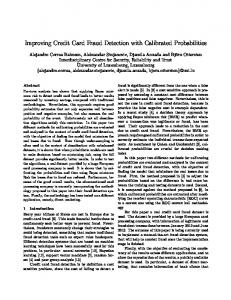
The Support Vector Machines (SVM) algorithm was first introduced by Cortes and Vapnik (1995). This algorithm finds a special kind of linear model, the maximum margin hyperplane, and it classifies all training instances correctly by separating them into correct classes through a hyperplane (a linear model). The maximum margin hyperplane is the one that gives the greatest separation between the classes – it comes no closer to any of the classes than it has to. The instances that are closest to the maximum margin hyperplane – the ones with minimum distance to it – are called support vectors. There is always at least one support vector for each class, and often there are more (Witten and Frank 2005). The optimal hyperplane is found by maximizing the width of the margin. As shown in Figure 2-1, the margin is the distance between the separating hyperplane and the closest positive class and negative class.

19

Figure 2-1: Separating two classes using a hyperplane (Leopold and Kindermann 2006)

In situations that the classes are not perfectly separable, the SVM algorithm finds the hyperplane that maximizes the margin while minimizing the misclassified instances using a slack variable. As shown in Figure 2-1, the slack variable, ξ, represents the distance of the misclassified instance from its margin hyperplane. The SVM algorithm minimizes the sum of distances of the slack variables from the margin hyperplanes while maximizing the margin width. This is done by solving the following equation using Quadratic Programming: 1 2 w  C  i 2 i 1 Minimize:

Subject to:

(2.7)

yi ( w  xi  b)  1  i , xi

i  0

Where w and b are parameters that are learned using the training data, ξ is the slack variable that represents the outliers, and C is a parameter that allows for selecting the complexity of the 20

model. The larger the C value is the less training errors are accepted and the more complex the predictive model becomes. There are situations where a nonlinear region can separate the classes more effectively. Rather than fitting nonlinear curves to the data, SVM determines a dividing line by using a kernel function to map the data into a different space where a hyperplane can be used to do a linear separation. The concept of a kernel mapping function is very powerful because it allows SVM models to perform separations even with very complex boundaries. An infinite number of kernel mapping functions can be used, but the Radial Basis Function has been found to work well for a wide variety of applications including credit card fraud (Hanagandi, Dhar and Buescher 1996). The transformation to a high-dimensional space is done by replacing every dot product in the SVM algorithm with the Gaussian radial basis function kernel as follows: K ( x i , x j )  exp(  || x i  x j || 2 ),   0

(2.8)

K ( xi , x j )   ( xi )   ( x j )

(2.9)

Where K(xi,xj) is the kernel function and φ(x) is the transformation function. 2.2.6

Neural Networks

Artificial Neural Networks (ANN) are computational models that try to mimic our body’s biological neural networks and can easily adapt to change. This mathematical model consists of interconnected artificial neurons (nodes) that can receive one or more inputs and sums them to produce a prediction (output). A neuron has two modes of operation: training mode, and usage mode. In training mode, the neuron can be taught to associate a certain prediction with an input

21

pattern. While in usage mode, if a taught input pattern is detected by the neuron its associated prediction is outputted. The effect of each input’s contribution to the final prediction is dependent on the weight of the particular input. To determine a neural network that is an accurate predictor, appropriate weights for the connections must be determined. The most widely used method to determine the optimal connection weights is called backpropagation. This method was introduced by Rumelhart, Hinton, and Williams (1986) and through their work artificial neural network research gained recognition in machine learning. Backpropagation utilizes a mathematical algorithm called gradient descent which iteratively adjusts a function’s parameters to minimize the squared error function of the network’s output. If the function has several minima the gradient descent method might not find the best one. The sigmoid function is used to calculate the output of each network layer and is defined as follows:

f ( x) 

1 1  ex

(2.10)

The squared error function is defined as follows:

E

1 ( y  f ( x)) 2 2

(2.11)

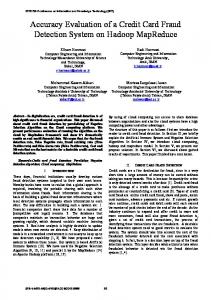
Where f(x) is the network’s prediction obtained from the output unit and y is the instance’s class label. An example of a neural network is shown in Figure 2-2.

22

Figurre 2-2: Exam mple of a neeural networrk with onee hidden layer

To find th he weights of o a neural network, n the derivative of the squaredd error functtion must bee determin ned. The derrivative of th he error functtion with resspect to a paarticular weigght is defineed as: dE  ( y  f ( x )) f ' ( x) a i dwi

((2.12)

Where wi are the weiights for the ith input varriable, x is thhe weighted sum of the iinputs, and ai are the inputs to the neurral network. This compu utation is reppeated for eaach training iinstance, andd the changes associated a with w a particu ular weight wi are added up, multipliied by the leearning rate ((a small con nstant), and subtracted frrom the wi’ss current valuue. This is reepeated untill the changes in the weigh hts become very v small.

23

2.2.7

Logistic Regression

Logistic regression is often used when the dependent variable takes only two values and the independent variables are continuous, categorical, or both. Logistic regression method is ideal when classifying outcomes that only have two values because the logistic curve is limited to values between 0 and 1. The method utilized in this thesis is based on the work done by le Cessie and van Houwelingen (1997). In credit card fraud detection the dependent variable would take on a value of 0 (legitimate transaction) or 1 (fraudulent transaction). Unlike ordinary linear regression however, logistic regression does not assume a linear relationship between the independent variables and the dependent variable, nor does it assume that the dependent variable or the error terms are distributed normally. The logistic regression model is defined as follows: p log( )   0  1 X 1   2 X 2  ...   k X k 1 p

(2.13)

Where X1,X2,…,Xk are the independent variables and p is the probability that the dependent variable has a value of 1.  0 is a constant and 1 ,…,  k are coefficients of the independent variables. The logistic regression model looks similar to the multi-linear regression equation, p however, the logistic regression regresses against the logit, log( ) , and not against the 1 p

dependent variable (See Figure 2-3). The Maximum Likelihood Estimation (MLE) is then used to compute the beta coefficients in the logistic regression formula. The aim of MLE is to find the parameter values that make the observed data most likely to be predicted. Likelihood and

24

probabiliity are closelly related because the lik kelihood of tthe parameteers given thee data is equaal to the probaability of thee data given the t parameteers (Montgoomery and Ru Runger 2003)). Likelih hood  Estiimating mod del parameteers given thee observed daata Pro obability  Predicting P an outcome ggiven model parameters The T likelihoo od function iss defined as follows: L(a )  f ( x1 ; a)  f ( x2 ; a )    f ( xn ; a )

((2.14)

ved values of o a dataset, a is a single unknown paarameter, annd Where x1,1 x2, …, xn arre the observ f(x;a) is the t probabiliity distributiion function.. The MLE aalgorithm iniitially choosses arbitrary numbers for the parameters, and through an iterative i pro cess the paraameters are slowly channged unction is maximized. m until the likelihood fu By B using the beta parameeters calculatted by the M MLE method and the corrresponding values off the indepen ndent variablles, the expeected probabbility for a fraaudulent trannsaction cann be calculated.

Fiigure 2-3: Comparison C n of the Lineear Probabiility model w with the Loggit Model 25

There are advantages and disadvantages with applying certain algorithms to fraud detection. Therefore a metric is needed to determine the ideal algorithms to use in the credit card fraud domain. A “diversity” value was selected as a metric to determine the optimal algorithms because it is easily calculated and the numerical score output can assist in ranking the best base algorithms to use as base classifiers. The diversity calculation method is discussed in detail in Chapter 4.

2.3

Introduction to Combination Strategies in Data Mining

The three main combination techniques used in data mining – bagging, boosting, and stacking – are presented in detail in this section. The bagging and boosting methods both use voting to combine the output of individual models of the same type (the same algorithm is used in constructing the models). However, boosting is an iterative process that uses weighted instances that focuses on a particular set of instances to build a prediction model. Stacking differs from both the boosting and bagging method because it combines the output of different types of algorithms to generate a final prediction. In the following section the bagging, boosting, and stacking techniques are discussed in detail and step-by-step examples are presented for these three combination techniques. All learning systems work by adapting to a specific environment. Given instances that have not been encountered, learning algorithms use their own set of assumptions to generate predictions. These assumptions are referred to as inductive bias (Mitchell 1980). Different algorithms have different representations and search heuristics, therefore, by using multiple algorithms, different search spaces can be explored and potentially diverse results can be obtained. No single algorithm works best on all kinds of datasets, therefore it is beneficial to use combinations of learning algorithms to evaluate complex databases. 26

There T are sev veral machine learning teechniques thhat have beenn developed to combine the output off different learning modeels. The three main technniques are: bbagging, booosting, and stacking. “Bagging” stands for bo ootstrap agg gregating andd was introdduced by Breeiman in 19996 (Breiman n 1996). This method usees training datasets d of thhe same size to produce m multiple classifierrs. These classifiers geneerate predictiions that aree used to deteermine the ffinal predictiion through the t process of o voting. Fo or each test instance eachh classifier ““votes” on w which class itt believes to be correctt (the classiffier’s predicttion), and thee class that rreceives the most “votess” is ng algorithm m is summariized in Figurre 2-4. The considereed to be the correct classs. The baggin uniqueneess of baggin ng is in the way w the train ning datasets are generateed. It is oftenn difficult orr expensiv ve to extract training t dataa from a com mplex domai n. Instead off obtaining iindependent datasets, bagging resamples the original o train ning data witth some of itts instances deleted and other d performs effectively e foor unstable leearning algoorithms wherre a instancess replicated. This method small chaange in the data d results in n a large chaange in preddictions.

Figure 2--4: Bagging algorithm as described bby (Witten and Frank 2005)

27

Freund and Schapire (199 96) introduceed an algoritthm called A AdaBoost whhich is considereed a “boostin ng” algorithm m. Boosting is an iterativve techniquee that uses vvoting to com mbine models of o the same ty ype (i.e. com mbining multiple decisioon trees). Thee learning allgorithm in tthis method is taught to concentrate c on o instances that are missclassified byy the previouus model by placing a larger emph hasis (weigh ht) on the misclassified innstances whhile decreasinng learning emphasiss on the corrrectly classiffied instances. A new claassifier is buuilt by learninng from the reweighted instancess, which focu uses on correectly classifyying the prevviously miscclassified m is summarrized in Figuure 2-5. As m mentioned prreviously, instancess. The boostiing algorithm boosting uses a votin ng system to determine a final predicction from thhe multiple m models of thee same typ pe. To make this final preediction the weights of aall classifierss that vote foor a particulaar class are summed, an nd the class with w the greaatest total weeight is chossen.

Figure 2-5: Boosting algorithm ass described bby (Witten aand Frank 2005).

28

Wolpert (1992) presented a novel technique in combining multiple models built by different learning algorithms termed stacked generalization, or stacking for short. Whereas bagging and boosting are used to combine models of the same type through the process of voting, stacking introduces the concept of a meta-learner that uses the predictions of different base models (the models that are to be combined) as input into its learning algorithm. The danger with using unweighted voting is the possibility of having multiple classifiers that are grossly incorrect which would lead to extremely inaccurate predictions. The meta-learner in the stacking technique is a separate learning algorithm that tries to learn which base classifiers are reliable. Meta-learning studies how to choose the right bias dynamically, as opposed to base-learning (single algorithm learning) where the bias is fixed or user parameterized. Meta-learning is a general technique to combine the results of multiple learning algorithms, each applied to a set of training data. 2.3.1

Examples using Meta-learning: Applying the bagging, boosting, and stacking methodologies

The dataset in Table 2-1 is used to show how the bagging, boosting, and stacking method are applied to produce final predictions. The dataset contains three attributes: transaction amount, transaction location, and type of credit card used for the transaction. The dataset also contains the correct class label for each transaction: either fraudulent or legitimate.

29

Table 2-1: Arbitrary training dataset consisting of three attributes with correct class Inst. #

1 2 3 4 5 6 7 8 9

Transaction Amount ($) 2 16 24 108 427 28 59 107 97

Transaction Location USA Canada Canada Canada Canada USA Canada Canada USA

Type of Credit Card Gold Gold Gold Platinum Platinum Platinum Gold Platinum Platinum

Correct Class

Fraud Legit Legit Fraud Legit Legit Legit Fraud Fraud

2.3.1.1 Bagging Example

Let us initially choose five random instances from the training dataset in Table 2-1, and randomly choose to replace two old instances with two new instances for each iteration. These new datasets – Table 2-2, Table 2-3, and Table 2-4 – are generated by re-sampling the original training data. Table 2-2: Bagging Dataset #1 Instance # 1 4 5 8 3

Transaction Amount ($) 2 108 427 107 24

Transaction Location USA Canada Canada Canada Canada

Type of Credit Card Gold Platinum Platinum Platinum Gold

Correct Class Fraud Fraud Legit Fraud Legit

Table 2-3: Bagging Dataset #2 Instance # 2 9 5 8 3

Transaction Amount Transaction Type of Credit ($) Location Card 16 Canada Gold 97 USA Platinum 427 Canada Platinum 107 Canada Platinum 24 Canada Gold *red represents new instances taken from original training dataset

30

Correct Class Legit Fraud Legit Fraud Legit

Table 2-4: Bagging Dataset #3 Instance # 2 9 6 7 3

Transaction Amount Transaction Type of Credit ($) Location Card 16 Canada Gold 97 USA Platinum 28 USA Platinum 59 Canada Gold 24 Canada Gold *red represents new instances taken from original training dataset

Correct Class Legit Fraud Legit Legit Legit

For this example a decision tree algorithm is selected as the training algorithm and is applied to bagging dataset #1, #2, and #3 to generate three different classification models – prediction models 1, 2, and 3. These models are applied to a testing dataset (Table 2-5). The predictions for each instance for each model are outputted and the majority prediction from the three models is then used as the final prediction as shown in Table 2-6. Table 2-5: Testing dataset consisting of new unclassified instances Instance #

100 101 102 103 104 105 106 107 108


31

Transaction Type of Location Credit Card USA Platinum USA Gold Canada Gold Canada Gold Canada Gold Canada Platinum USA Gold Canada Gold USA Platinum

Table 2-6: Applying the three bagging models to a testing dataset Inst. Transaction Transaction # Amount ($) Location

100 101 102 103 104 105 106 107 108

251 12 59 1005 432 29 65 803 25

USA USA Canada Canada Canada Canada USA Canada USA

Type of Credit Card Platinum Gold Gold Gold Gold Platinum Gold Gold Platinum

Prediction from Model #1 Fraud Fraud Legitimate Legitimate Fraud Legitimate Fraud Fraud Legitimate

Prediction from Model #2 Fraud Legitimate Legitimate Legitimate Legitimate Fraud Fraud Fraud Legitimate

Prediction from Model #3 Fraud Legitimate Fraud Legitimate Fraud Legitimate Legitimate Fraud Legitimate

Final Class Prediction Fraud Legitimate Legitimate Legitimate Fraud Legitimate Fraud Fraud Legitimate

As can be seen from Table 2-6, the final prediction in the bagging method is based on a majority vote from the predictions of models 1, 2, and 3. 2.3.1.2 Boosting Example

Once again we use the data presented in Table 2-1, however for the boosting methodology there are weights associated with each instance. Before the iterative procedure begins, each training instance is assigned an equal random weight as shown below in Table 2-7 (a positive number between zero and infinity is randomly picked as the starting weights). Table 2-7: Boosting Dataset Example Instance #

1 2 3 4 5 6 7 8 9


Transaction Location USA Canada Canada Canada Canada USA Canada Canada USA

32


Correct Class Fraud Legit Legit Fraud Legit Legit Legit Fraud Fraud

Weights

0.6 0.6 0.6 0.6 0.6 0.6 0.6 0.6 0.6

Boosting Iteration #1:

Let us assume that we apply a decision tree algorithm to Table 2-7 in which all instances have equal weights, to generate a classification model that outputs a prediction for each instance. The root mean squared error (RMSE) term for the classifier, e (a fraction between 0 and 1), is then calculated using the following formula:

e

 (x

i

 yi )

2

n

(2.15)

Where xi is the predicted probability outcome of instance i, yi is the actual outcome of instance i, and n is the number of instances under investigation . For correctly classified instances, the weight of each instance is adjusted by the following formula:

Adjusted Weight  Weight 

e (1  e)

(2.16)

Where e is the error term for the classifier. Weights remain unchanged for misclassified instances. All weights are then normalized by dividing each instance’s weight by the sum of the new weights and multiplying by the sum of the old weights. Assuming the error term for this classifier is 0.35, the adjusted weights for each instance can be calculated using Equation 2.16. Table 2-8 shows the adjusted and normalized weights for each instance.

33

Table 2-8: Boosting iteration #1 Instance Txn Transaction Type of Correct Weights Classified Adjusted Normalized # Amt Location Credit Class #1 Weights Weights ($) Card 1 2 USA Gold Fraud 0.6 Correctly 0.323 0.434 2 16 Canada Gold Legit 0.6 Correctly 0.323 0.434 3 24 Canada Gold Legit 0.6 Incorrectly 0.6 0.807 4 108 Canada Platinum Fraud 0.6 Correctly 0.323 0.434 5 427 Canada Platinum Legit 0.6 Incorrectly 0.6 0.807 6 28 USA Platinum Legit 0.6 Correctly 0.323 0.434 7 59 Canada Gold Legit 0.6 Incorrectly 0.6 0.807 8 107 Canada Platinum Fraud 0.6 Incorrectly 0.6 0.807 9 97 USA Platinum Fraud 0.6 Correctly 0.323 0.434

As shown in Table 2-8, the weights of correctly classified instances are decreased while weights are increased for incorrectly classified instances. Boosting Iteration #2:

For the second iteration in the boosting methodology, the decision tree algorithm is applied to the original dataset from Table 2-7 but with the new adjusted weights calculated from iteration #1 (See the red numbers in Table 2-8) instead of the original weights. This produces a second classification model with its own set of predictions. The weights are once again adjusted and normalized to put more emphasis on incorrectly classified instances. Assuming the error term for the classifier for this iteration is 0.30, the weights from iteration #1 are adjusted using Equation 2.16 to calculate new adjusted weights for each instance (See Table 2-9).

34

Table 2-9: Boosting iteration #2 Inst. #

1 2 3 4 5 6 7 8 9

Txn Amt ($) 2 16 24 108 427 28 59 107 97

Txn Location

USA Canada Canada Canada Canada USA Canada Canada USA


Correct Class


Weights #2 (from #1) 0.434 0.434 0.807 0.434 0.807 0.434 0.807 0.807 0.434

Classified

Correctly Incorrectly Incorrectly Correctly Correctly Correctly Incorrectly Incorrectly Correctly

Adjusted NormalWeights ized Weights 0.186 0.255 0.434 0.594 0.807 1.104 0.186 0.255 0.346 0.473 0.186 0.255 0.807 1.104 0.807 1.104 0.186 0.255


Once again the decision tree algorithm is applied to the original dataset (Table 2-7), but the weights are the adjusted weights from the previous iteration (iteration #2 – see the blue numbers from Table 2-9). This produces a third classification model with its own set of predictions. The weights are once again adjusted using Equation 2.16 and then normalized. Assuming the error term for the classifier for this iteration is 0.15, the data from Table 2-10 can then be constructed.

35

Table 2-10: Boosting iteration #3 Txn Amt ($) 2 16 24 108 427 28 59 107 97

Txn Location



Correct Class

Weights #3 (from $2)

Classified

Adjusted Weights

Normalized Weights


0.255 0.594 1.104 0.255 0.473 0.255 1.104 1.104 0.255

Correctly Incorrectly Incorrectly Correctly Incorrectly Correctly Correctly Correctly Incorrectly

0.045 0.594 1.104 0.045 0.473 0.045 0.195 0.195 0.255

0.082 1.087 2.020 0.082 0.865 0.082 0.357 0.357 0.467


The decision tree algorithm is applied to the dataset with the new weights calculated from the previous iteration (iteration #3) to generate a fourth prediction model. However, let us assume that the overall error for this model is zero, therefore the fourth prediction model is not created. In the boosting methodology, whenever the error term is zero, or when it is greater or equal to 0.5, the iterative process stops and no more models are constructed. Therefore, in this example the boosting method stops after three iterations.

Final Prediction:

For the final classification of an instance in the boosting method, the weights of all classifiers that vote for a particular class are summed and the class with the greatest total is chosen to be the final prediction. The process begins by assigning a weight of zero to all classes (fraud or legit). For each instance a  log

e term is added to the weight of a class predicted by 1 e

36

a model. The class with the highest weight is chosen as the final prediction. The three boosting models from this example are applied to a new testing dataset (dataset originally introduced in Table 2-5) and the predictions for each instance using these models are determined (See Table 2-11). The weights associated with each model for each instance, the sum of the weights for each class, and the final prediction for each instance using the boosting method are shown in the following Table 2-11. Table 2-11: Using the three boosting models to determine the final predictions

Inst. #

100 101 102 103 104 105 106 107 108

Model Model Model #1 #2 #3 Predicts Predicts Predicts Fraud Fraud Fraud Legit Fraud Fraud Legit Legit Legit Legit Legit Legit Fraud Legit Legit Fraud Fraud Fraud Legit Legit Fraud Fraud Fraud Legit Legit Legit Fraud

Class Weights (  log

e ) 1 e

Model #1 e=0.35 0.269 0.269 0.269 0.269 0.269 0.269 0.269 0.269 0.269

Model #3 e-0.15 0.753 0.753 0.753 0.753 0.753 0.753 0.753 0.753 0.753

Model #2 e=0.30 0.368 0.368 0.368 0.368 0.368 0.368 0.368 0.368 0.368

Weighted Vote Fraud Legit

1.39 1.121 0 0 0.269 1.39 0.753 0.637 0.753

0 0.269 1.39 1.39 1.121 0 0.637 0.753 0.637

Final Predict

Fraud Fraud Legit Legit Legit Fraud Fraud Legit Fraud

In summary, the boosting method is an iterative process in which the weights of correctly classified instances are decreased and the weights of misclassified instances are increased. This produces classifiers that focus on classifying instances that were previously misclassified. The final prediction is determined by a weighted vote in which the predictions from well performing classifiers have greater influence in the voting process.

37

2.3.1.3 Stacking Example

Bagging and boosting combine models of the same type to produce a final prediction, on the other hand, stacking applies models built by different learning algorithms. Instead of voting, stacking introduces a meta-classifier which tries to learn which classifiers (base classifiers) are the reliable ones using another learning algorithm. This meta-classifier tries to determine the best way to combine the outputs of the base classifiers. The k-nearest neighbour algorithm (kNN), rule-based algorithm, and Bayesian algorithm are used to construct the base classifiers. The decision tree algorithm is used to construct the meta-classifier (classifier generated using the meta-learner algorithm). Table 2-12 consists of the same data from Table 2-1 but with a separation of the instances into either training data for the base classifiers or training data for the meta-classifier. Two-thirds of the data in Table 2-12 is used for training the base classifiers, while the remaining one-third is used for training the metaclassifier.

Table 2-12: Base classifier predictions on the example dataset Instance # Transaction Transaction Type of Amount ($) Location Credit Card

1 2 3 4 5 6 7 8 9

2 16 24 108 427 28 59 107 97


Gold Gold Gold Platinum Platinum Platinum Gold Platinum Platinum

38

Correct Class


Training data for base or meta classifier Base classifiers Base classifiers Base classifiers Base classifiers Base classifiers Base classifiers Meta-classifier Meta-classifier Meta-classifier

The chosen base algorithms are applied to the base classifiers’ training data to generate base classification models. These models are applied to the meta-classifier training data to output predictions that are used as new attributes to the meta-classifier’s training data (See Table 2-13). Table 2-13 shows the modification of the meta-classifier training dataset by using the predictions of the base classifiers as new attributes and combining them with the data that was originally set aside to train the meta-classifier. Table 2-13: Base classifier predictions as new attributes in the meta-classifier training data Transaction Amount ($)

Transaction Location

59 107 97

Canada Canada USA

Type of Credit Card Gold Platinum Platinum

kNN

Rulebased

Bayesian

Fraud Legit Legit

Fraud Fraud Legit

Fraud Fraud Fraud

The meta-classifier algorithm is applied to the data in Table 2-13 (the decision tree algorithm is chosen as the meta-classifier algorithm in this example) to construct the metaclassifier model that produces the final predictions. Table 2-14 shows the final meta-classifier prediction for a new testing dataset originally introduced in Table 2-5. Table 2-14: Applying the meta-classifier model to a new testing dataset Instance #

Transaction Amount ($)

Transaction Location

Type of Credit Card

100 101 102 103 104 105 106 107 108

251 12 59 1005 432 29 65 803 25

USA USA Canada Canada Canada Canada USA Canada USA

Platinum Gold Gold Gold Gold Platinum Gold Gold Platinum

39

Metaclassifier prediction Fraud Fraud Legit Legit Legit Legit Fraud Legit Fraud

The meta-classifier prediction does not select the majority prediction from the base classifiers. The meta-classifier uses its own algorithm to select the best prediction based on the predictions of the base classifiers.

In summary, there are many different algorithms that are capable of detecting credit card fraud. These algorithms can use either supervised or unsupervised learning and can range from statistical methods such as the Bayesian algorithm, to perceptron-based algorithms such as a neural network. The method of combining models aims to combine the strengths of different algorithms to improve the accuracy of fraud detection and is just one of the many techniques that have been used in literature for credit card fraud detection. The next chapter outlines the wide range of techniques that have been used in the past to detect different types of fraud.

40

3

Literature on Credit Card Fraud Detection

In this chapter a detailed literature study of the different techniques in fraud detection are presented. Section 3.1 outlines the methodologies used in literature for the detection of fraud using single or multi-algorithm based prediction models. The literature review in Section 3.1 is presented in chronological order. The following section, Section 3.2, introduces meta-learning (a multi-algorithm technique) and discusses the latest work in credit card fraud that have used this technique. Finally Section 3.3 describes in detail the specific process of meta-learning, the Combiner Strategy, that is implemented in this thesis for the construction of the meta-classifier.

3.1 Single and Multi-Algorithm Techniques for Fraud Detection used in Literature Many techniques have been applied to the field of fraud detection ranging from supervised learning and unsupervised learning to hybrid models. Bolton and Hand (2001), and Kim, Ong and Overill (2003) both used outlier detection methods to detect abnormality in credit card transactions. Outlier detection techniques are unsupervised learning approaches that do not require prior knowledge of fraudulent and non-fraudulent transactions in historical databases. These techniques look for observations that deviate from other observations as to arouse suspicion. The advantage of unsupervised methods is that previously undiscovered types of fraud may be detected. Supervised methods require accurate identification of fraudulent transactions and are only trained to discriminate between legitimate transactions and previously known fraud. However, outlier detection can cause legitimate erratic behavior to be classified as an anomaly, thus causing inconveniences to the customer. A more sophisticated method that is used often in literature and industry is neural networks. Neural networks are made up of interconnected nodes that try to imitate the functioning of the human brain. Each node has a weighted connection to several other nodes in adjacent layers. Individual nodes take the input received from connected 41

nodes and use the weights together with a simple function to compute output values. The neural network method can be either supervised or unsupervised and the output layer may contain one or several nodes. Other methods seen in literature that have been used to detect fraud include rule-based systems, decision trees, support vector machines, meta-classifier systems, and other data mining methods, as discussed below. Ghosh and Reilly (1994) used a neural network system which consists of a three-layered feed-forward network with only two training passes to achieve a reduction of 20% to 40% in total credit card fraud loses. This system also significantly reduced the investigation workload of the fraud analysts. Aleskerov, Freisleben, and Rao (1997) developed a fraud detection system called Cardwatch that is built upon the neural network learning algorithm. This system is aimed towards commercial implementation and therefore can handle large datasets, and parameters of an analysis can be easily adjusted within a graphical user interface. Cardwatch uses three main neural network learning techniques: conjugate gradient, backpropagation, and batch backpropagation. This system is a useful product for large financial institutions due to its ease of implementation with commercial databases. Unfortunately, the disadvantage of this system is the need to build a separate neural network for each customer. This results in a very large overall network that requires relatively higher amounts of resources to maintain. Dorronsoro, and others (1997) developed a neural network based fraud detection system called Minerva. This system’s main focus is to imbed itself deep in credit card transaction servers to detect fraud in real-time. It uses a novel nonlinear discriminant analysis technique that 42

combines the muti-layer perceptron architecture of a neural network with Fisher’s discriminant analysis method. Minerva does not require a large set of historical data because it acts solely on immediate previous history, and is able to classify a transaction in 60ms. The disadvantage of this system is the difficulty in determining a meaningful set of detection variables and the difficulty in obtaining effective datasets to train with. Kokkinaki (1997) suggested to create a user profile for each credit card account and to test incoming transactions against the corresponding user’s profile. The attributes that were used to construct these profiles are: credit card numbers, transaction dates, type of business, place, amount spent, credit limit and expiration time. Kokkinaki proposed a Similarity Tree algorithm, a variation of Decision Trees, to capture a user’s habits. The analyses found that the method has a very small probability for false negative errors. However, in this approach the user profiles are not dynamically adaptive and therefore continual updates are needed when user habits and fraud patterns change. Chan and Stolfo (1998) studied the class distribution of a training set and its effects on the performance of multi-classifiers on the credit card fraud domain. It was found that increasing the number of minority instances in the training process results in fewer losses due to fraudulent transactions. Furthermore, the fraud distribution for training was varied from 10% to 90% and it was found that maximum savings were achieved when the fraud percentage used in training was 50%. Brause and others (1999) looked specifically at credit card payment fraud and identified fraud cases by combining a rule-based classification approach with a neural network algorithm. In this approach the rule-base classifier first checked to see if a transaction was fraudulent, and

43

then the transaction classification was verified by a neural network. This technique increases the probability for the diagnosis of “fraud” to be correct and therefore it is able to decrease the number of false alarms while increasing the confidence level. Ehramikar (2000) showed that the most predictive Boosted Decision Tree classifier is one that is trained on a 50:50 class distribution of fraudulent and legitimate credit card transactions. It was also reported that training decision tree classifiers on datasets with a high distribution of legitimate transactions leads to high fraudulent cases classified as legitimate (a high false negative rate). This suggests that predictive model over fitting occurs when the training dataset has a majority of legitimate transactions.

Wheeler and Aitken (2000) developed a case-based reasoning system that consists of two parts, a retrieval component and a decision component, to reduce the number of fraud investigations in the credit approval process. The retrieval component uses a weighting matrix and nearest neighbor strategy to identify and extract appropriate cases to be used in the final diagnosis for fraud, while the decision component utilizes a multi-algorithm strategy to analyze the retrieved cases and attempts to reach a final diagnosis. The nearest-neighbour and Bayesian algorithms were used in the multi-algorithm strategy. Initial results of 80% non-fraud and 52% fraud recognition from Wheeler and Aitken suggest that their multi-algorithmic case-based reasoning system is capable of high accuracy rates. Bolton and Hand (2001) proposed an unsupervised credit card detection method by observing abnormal spending behaviour and frequency of transactions. The mean amount spent over a specified time window was used as the comparison statistic. Bolton and Hand proposed the Peer Group Analysis (PGA) and the Break Point Analysis (BPA) techniques as unsupervised 44

outlier detection tools. The paper showed that the PGA technique is able to successfully detect local anomalies in the data, and the BPA technique is successful in determining fraudulent behaviour by comparing transactions at the beginning and end of a time window. Kim (2002) proposed a fraud density map technique to improve the learning efficiency of a neural network. There is an overemphasis of fraudulent transactions in training data sets, therefore, the fraud density map (FDM) tries to address the issue of the inconsistent distributions of legitimate and fraudulent transactions between the training data and real data. FDM adjusts the bias found in the training data by reflecting the distribution of the real data onto the training data through the changing of a weighted fraud score. Maes (2002) applied artificial neural networks (ANN) and Bayesian belief networks (BBN) to a real world dataset provided by Europay International. The best prediction rate was obtained for the experiment in which the features were pre-processed. It was found that by performing a correlation analysis on the features and removing the feature that was strongly correlated with many of the other features clear improvements to the results were obtained. Furthermore, their experiments showed that BBNs yields better fraud detection results and their training period is shorter, however ANN was found to be able to compute fraud predictions faster in the testing stage. Chen and others (2004) presented a new method to address the credit card fraud problem. A questionnaire-responded transaction (QRT) data of users was developed by using an online questionnaire. The support vector machine algorithm was then applied to the data to develop the QRT models, which were then used to decide if new transactions were fraudulent or legitimate.

45

It was found that even with very little transaction data the QRT model has a high accuracy in detecting fraud. Chiu and Tsai (2004) identified the problem of credit card transaction data having a natural skewness towards legitimate transactions. The ratio of fraud transactions to normal transactions is extremely low for an individual FI, and this makes it difficult for FIs to maintain updated fraud patterns. The authors of this paper proposed web service techniques for FIs to share their individual fraud transactions to a centralized data centre and a rule-based data mining algorithm was then applied to the combined dataset to detect credit card fraud. Fan (2004) proposed an efficient algorithm based on decision trees. The decision tree “sifts through” old data and combines it with new data to construct the optimal model. The basic idea is to train a number of random and uncorrelated decision trees, and each decision tree is constructed by randomly selecting available features. The structure of the trees are uncorrelated, the only correlation is in the training data itself. Foster and Stine (2004) attempted to predict personal bankruptcy using a fully automated stepwise regression model. Neural network models used in fraud detection modeling are often regarded as black-boxes, and it is difficult to follow the process from input to the output prediction. On the other hand, the benefit of a statistical model is the ability to easily understand the procedures in the prediction process. The results from this paper indicate that standard statistical models are competitive with decision trees. Abdelhalim and Traore (2009) tackled the application fraud problem where a fraudster applies for an identity certificate using someone else’s identity. Identity certificates were extracted from the web and cross-referenced with the information from application forms and identity claims (i.e. passport application, credit card application, etc.) to detect anomalies. The 46

paper introduced a rule-based decision tree technique to design their fraud detector. This technique was able to correctly identify 92% of the application fraud cases. The single algorithm techniques presented above are summarized in Table 3-1, while the multi-algorithm techniques used in literature are summarized in Table 3-2. These experiments show that in the study of fraud activities, neural networks, Bayesian algorithms, decision trees, and nearest-neighbour methods are extremely effective in fraud detection. The neural network methodology has been found to be the most popular method in recent credit card fraud detection studies (Ngai, et al. 2011), however, there also has been successful work in literature on fraud identification using different algorithms such as decision trees, statistical models, and nearestneighbour strategies (See Table 3-1). The effectiveness of these algorithms led to the selection of a multi-algorithm strategy to detect credit card fraud for this thesis. By applying multiple algorithms onto a neural network filtered dataset we hope to further improve the accuracy of fraud detection. Studies have shown that Bayesian networks and regression models are able to outperform neural networks in fraud detection accuracy. The study of combining different data mining algorithms have also increased in literature and have shown to outperform single algorithm methods. Since the dataset in this thesis consists of transactions that have already been filtered by a neural network model, a multi-algorithmic approach that consists of algorithms other than a neural network has the greatest potential in improving fraud detection and therefore a multialgorithm method is used in this thesis.

47

Table 3-1: Summary of single algorithm techniques in literature for the prediction of fraud Reference Ghosh and Reilly (1994)

Method Neural network (restricted coulomb energy algorithm)

Aleskerov, Freisleben, and Rao (1997) Dorronsoro (1997)

Neural network (gradient descent algorithm) Neural network

Kokkinaki (1997)

Decision tree

Ehramikar (2000)

Decision tree

Wheeler and Aitken (2000)

Case-based reasoning (Nearest neighbor and probabilistic algorithms)

Bolton and Hand (2001)

Outlier detection (unsupervised)

Method Applied to: Advantages Credit card transactions Increased accuracy and timeliness of fraud detection

Disadvantages Compared to other data mining techniques this method requires a longer training period Credit card transactions Can handle large commercial Non-convergence in size databases training

Credit card transactions Real-time fraud detection

Credit card transactions Simple and easy to implement; reduced misclassifications Credit card transactions Predictive performance was improved by increasing the number of minority instances Credit applications Model can be easily updated and maintained; robust to missing or irrelevant data

Credit card transactions Successful in detecting local anomalies and can detect fraudulent behavior in a continuous manner 48

Difficulty in determining the optimal size of the hidden layers Not dynamically adaptive Only the decision tree algorithm is experimented upon Requires two separate experiments; one to determine the instances to experiment upon, and another to determine the final prediction. Treats all accounts equally; does not differentiate between different accounts

Kim (2002)

Neural network with weighted fraud scores (unsupervised)

Credit card transactions Increased number of detected frauds compared to a neural network only classifier

Maes (2002)

Neural & Bayesian belief networks

Credit card transactions By removing highly correlated attributes, fraud detection was improved

Fan (2004)

Decision tree

Synthetic data and credit card transaction data

The use of a cross-validation decision tree ensemble decreases error rate in fraud prediction

Foster and Stine (2004)

Regression model

Personal bankruptcy

Easy to understand the procedure in the prediction process; competitive to neural networks and decision tree methods

49

Backpropagation is used to train the neural networks; this method is only able to find local minima in the error function, therefore an optimal model may not always be reached Bayesian algorithm performs better than neural networks in fraud detection Prediction performance with this method decreases as the percentage of recent transactions increase in the training data Linear models cannot easily adapt to changes in fraud patterns

Table 3-2: Summary of multi-algorithm techniques in literature for the prediction of fraud Reference Chan and Stolfo (1998)

Method Multi-classifier metalearning

Method Applied to: Credit card transactions

Brause (1999)

Combination of rule-based and neural network algorithms

Credit card transactions

Chen (2004)

Support vector machine applied to questionnaireresponded transaction data

Credit card transactions

Chiu and Tsai (2004)

Credit card Rule-based algorithm transactions applied to a web-based knowledge sharing scheme

Abdelhalim and Traore (2009)

Decision tree algorithm applied to online identity application data

Identity application fraud

50

Advantages A 46% improvement over the no fraud detection scenario was achieved

Disadvantages Required to determine the best distribution to use for each training experiment Batch process; requires Increased the number of correct classifications and two separate experiments (one for a rule-based decreased the number of algorithm and another for false alarms a neural network) New questionnaires need Able to achieve high accuracy in fraud detection to be conducted with very little transaction whenever user behaviour changes data Subject to the willingness Able to centralize of FIs to share credit card fraudulent transactions from different FIs, thereby transaction data increasing the prediction accuracy of models by training on a higher fraud distributed dataset The data used was a mix Able to correctly classify of real data collected 92% of the identity online and synthetic data; application fraud cases a more accurate experiment would be to use 100% real data

3.2

Meta-Learning in Credit Card Fraud Detection

This section outlines the development of the multi-algorithm strategy. The development of this strategy for credit card fraud began with its introduction in speech recognition and eventually was adapted for use in the credit card fraud detection. Meta-learning is a general technique to coalesce the results of multiple learners. The idea of applying multiple algorithms to achieve an overall accuracy higher than a single learning algorithm was first proposed in speech recognition by Stolfo, Galil, McKeown, and Mills in 1989 (Stolfo, et al. 1989). The first foray into the combiner strategy was studied by Wolpert (Wolpert 1992) who proposed a strategy to improve the cross-validation method by estimating and correcting for the error of a base classifier termed stacked generalization. The first foray into the arbiter strategy was conducted by Schapire (1990) and was termed “hypothesis boosting”. This scheme consists of three different classifiers. The first classifier learns from the given training data and generates its predictions. The second classifier learns from instances that are equally likely to be correctly or incorrectly classified by the first learned classifier. Finally, the last classifier is the arbiter classifier, this classifier learns from examples where both the first two classifiers disagree. The final prediction is chosen by analyzing the predictions of all three classifiers with the arbiter classifier breaking a tie in situations where the first two classifiers disagree. Schapire’s hypothesis boosting is essentially a boosting technique that requires the generation of two additional distributions of examples and utilizes only a single learning algorithm. Chan and Stolfo (1993) expanded Wolpert’s and Schapire’s initial works by developing a multistrategy hypothesis boosting technique that uses ideas from hypothesis boosting and stacked generalization. Three strategies are introduced: combiner strategy, arbiter strategy, and a hybrid

51

strategy. Each strategy has a different technique for combining the predictions of the base learners. The combiner strategy joins the predictions from the base classifiers by learning the relationship between base predictions and the correct prediction. The arbiter strategy learns from examples that are confusing to the base classifiers. Finally, the hybrid strategy picks examples as in the arbiter strategy (predictions that do not agree) and then joins the predicted classifications of data in disagreement by the base classifiers as in the combiner strategy. From the Chan and Stolfo experiments (Chan and Stolfo 1993) it was found that the combiner strategy performed more effectively than the arbiter or hybrid strategies. Credit card fraud detection using meta-learning strategies was first extensively studied by Stolfo and others (Stolfo, et al. 1997). Their initial results show that a meta-classifier generated using the Bayesian algorithm achieves the highest True Positive rates (correctly classified fraudulent transactions), while the best base classifiers are the ones generated using the CART and RIPPER algorithms. In a 1999 paper by Chan, a cost model was developed to evaluate the effectiveness of the meta-learning strategy proposed by Chan in 1993 (Chan and Stolfo 1993). The technique of combining multiple base models to produce meta-classifiers was used to offset the loss of predictive performance that usually occurs when mining from data subsets or sampling. The results from the experiments by Stolfo and Chan showed great success in the implementation of a meta-learning classifier in the detection of credit card fraud. The metalearning approach was shown to be significantly more effective than the methods used by the FIs at that time. Due to these findings, the meta-learning strategy was selected to be implemented onto the neural network filtered dataset.

52

3.3 Meta-Learning and the Combiner Strategy The methodology applied in the thesis work closely follows the “meta-learning” techniques introduced by Chan and Stolfo (Chan and Stolfo 1993). No single learning algorithm can uniformly outperform other algorithms over all datasets. Furthermore, previous studies have found that by modifying the distribution of examples in such a way as to force a learning algorithm to focus on the harder-to-learn parts of the distribution, the accuracy of this learner can be greatly improved (Schapire 1990). Thus, the meta-learning technique aims to coalesce the results of multiple learners to improve prediction accuracy and to utilize the strengths of one method to complement the weakness of another. In this approach, rather than using weights to train a model, the predictions of a set of base classifiers are used as training data to “meta-learn” a set of new classifiers. It involves applying multiple algorithms on the same dataset and combining the results by meta-learning. There are two methods of combing algorithms that were introduced by Chan and Stolfo, the arbiter and the combiner strategies. Through experimentation conducted in previous papers it was found that the combiner strategy performs more effectively than the arbiter strategy, therefore only the combiner strategy is used in this thesis. The next section provides an overview of the combination method used in the metalearning method (the “combiner strategy”).

53

3.3.1

The Combiner Strategy in Detail

In the combiner strategy, as shown in Figure 3-1, the attributes and correct classifications of credit card transaction instances are used to train multiple base classifiers. The predictions of the base classifiers are used as new attributes for the meta-level classifier. By combining the original attributes, the base classifier predictions, and the correct classification for each instance (the composition rule), a new “combined” dataset is created which is used as the training data to generate the meta-level classifier. The predictions from the meta-level classifier are then used as the final predictions in the combiner strategy.

Figure 3-1: Classification of a credit card transaction by the combiner strategy

54

In summary, the non-neural network techniques that have been used in literature for fraud detection were studied extensively in the late 1990’s and early 2000’s, furthermore, the metalearning strategy was last implemented on credit card data in 1999. Therefore it is valuable to determine the effectiveness of these techniques on recent credit card data. Results from the Chan and Stolfo studies have shown that the ‘Combiner Strategy’ is the best performing meta-learning method and this strategy is used exclusively in this thesis. In the next chapter the metrics used for the selection of the base classifiers, and the training, validation, and testing dataset sizes are discussed. The application of the combiner strategy and the performance evaluation using different ranking and evaluation methods are also described.

55

4

Methodology

In this Chapter, the methodologies used in the construction of the meta-classifier are discussed in detail. In Section 4.1, the software used in the construction of the meta-classifier is presented. Section 4.2 discusses in detail the filtering and pre-processing of the initial dataset, and the reasoning behind the construction of datasets with a 50:50 fraudulent to legitimate transaction ratio are presented. In Section 4.3 a metric is introduced to determine the optimal number of base classifiers, and the reasoning behind the selection of the types of algorithms used for the base classifiers are discussed. The next section, Section 4.4, discusses the selection of the training, validation, and testing dataset sizes. Section 4.5 presents the four stages involved in the construction of the meta-classifier. Finally Section 4.6 describes the ranking methods and the evaluation techniques used to determine the performance of the meta-classifier. 4.1

Software Used

All the meta-classification models and outputs were obtained using the open source “Weka” data mining software (Hall, et al. 2009). Weka is an open source program that contains a large set of data mining algorithms and is a program that is widely used in academia. The prime reason for choosing Weka is the abundance of algorithms that can be used and because the implementation of each algorithm is thoroughly documented in the software. Weka was developed and is maintained by the University of Waikato, in New Zealand. In addition to Weka, Microsoft Excel and SPSS Clementine software were used extensively for analyses throughout the experiments. 4.2

Data preparation

The dataset received from the FI contained transactions with Falcon scores ranging from 0 to 999. However, all transactions with a Falcon score lower than 900 were removed. By analyzing transactions only with high Falcon scores, the dataset is limited to transactions that are most 56

likely to be fraudulent. As a result, the percentage of minority instances is increased which is beneficial in the training process. The dataset for the testing month used in this thesis is from October 2009 and it contains 106,934 credit card transactions with Falcon scores greater than or equal to 900. For this testing month, 11,317 transactions have been verified by the FI as fraudulent and accounts for 10.6% of the transactions in this month. It is also important to point out the types of transactions that were present in this dataset. All credit card transactions go through a neural network system (Falcon fraud manager) as described in Section 1.1. Based on the Falcon score values, the FI’s in-house methods are then used to predict whether a transaction is legitimate or fraudulent. The dataset that is used throughout this paper is assumed to consist entirely of transactions that were deemed to be fraudulent by the FI classification methods (Falcon scores greater than 900). The correct classification labels are assumed to be determined through the investigation of these transactions. The dataset that was initially received from the FI contained 11 months of data from December 2008 to October 2009 with one data file per month. Each of these 11 files contained 41 attributes (See Appendix B: Table B1). After pre-processing and data cleansing, 29 attributes remained in the dataset (See Appendix B: Table B2). The “Time” and “Date” attributes themselves do not provide valuable classifier training information, however, the time and day differences between subsequent transactions can be quite informative. The “Time and “Date” attributes were converted to a more useful attribute by computing the difference in time and days between subsequent credit card transactions using the SPSS Clementine software. The “Time Difference” and a “Date Difference” attributes were generated to replace the “Time” and “Date” attributes respectively. The final major modification to the dataset was done to the merchant state attribute. Originally “Merchant State” consisted of the abbreviations for the 50 states of the 57

United States and the 10 provinces and 3 territories of Canada. This resulted in too many unique instances in the dataset, which could possibly weaken the predictive accuracy of the metaclassifier. Therefore, the 50 states were converted and reduced to just 4 labels depending on the region the state resided in. The 4 labels are: NEUS (North Eastern United States), MWUS (MidWestern United States), WUS (Western United States), and SUS (Southern United States) (Reasons for the removal and changes of attributes are listed in Appendix B: Table B3). The next step in the data preparation process was to match the credit card transactions to the FI’s database of verified fraudulent transactions. This was done by comparing the cleansed dataset that has 29 attributes with a new dataset that contained only fraudulent transactions. Using a C-program, the credit card number, time stamp, and date stamp were compared between the two datasets. If any matches were found, the program would add a ‘Y’ label to the transaction in the cleansed dataset to represent a fraudulent transaction. The final step in data preparation involved the removal of characters that were unacceptable for the Weka program. This was done by another C-program that would scan through the dataset and replace the unacceptable characters with dashes. The final 29 attributes used in the analysis for this thesis are listed in Appendix B: Table B4. The formatting of the attributes, whether the attributes were categorical or numerical, the possible values, and a brief description of each attribute are also listed in this table. In credit card fraud detection, it has been shown that the desired fraud to legitimate distribution is 50:50 for the training process (Ehramikar 2000), (Stolfo, et al. 1997). Therefore, the training datasets were divided into subsets such that 50% of the instances were fraudulent transactions and the other 50% were legitimate transactions (See Figure 4-1). The distribution of the original credit card datasets contained a 10:90 ratio of fraudulent to legitimate transactions. To achieve the desired 50:50 distribution, the minority instances were replicated across the 58

majority instances by dividing the dataset into partitions. The technique used to determine the number of partitions is as follows:

Number of Partitions =

y u  x v

(4.1)

Number of Minority Instances in each Partition = nx

(4.2)

nxv u

(4.3)

Number of Majority Instances in each Partition =

Where n is the size of the dataset with a distribution of x:y, x is the percentage of the minority instances, y is the percentage of the majority instances, u:v is the desired distribution where u is the desired percentage of minority instances, and v is the desired percentage for the majority instances. Since the original dataset contained approximately 10%fraudulent transactions and 90%legitimate transactions and the desired training dataset distribution is 50:50, the desired number of partitions was calculated to be nine (

90 50  ). The data subsets were formed by 10 50

merging the replicated minority instances (fraud transactions) with each of the 9 partitions containing majority instances (legitimate transactions) (Chan and Stolfo 1998).

59

Figure 4-1: Constructing a 50:50 distribution for the training datasets

4.3 Diversity – Selecting base classifiers The number of base classifiers used for the training stage and the type of algorithms used for each classifier were chosen based on a diversity metric as introduced by Chan (Chan 1996). This entropy-based metric measures the “randomness” of the predictions and how “different” the base classifiers are based on their predictions. It measures the average amount of information required to represent each event. The larger the diversity value, the more evenly distributed the predictions are for the base classifiers, while a smaller diversity value represents base classifiers that have predictions that have more bias (some predictions are more likely to occur) (Chan 1996). For each instance, yi, the fraction of base classifiers predicting class, classk, (pik) is calculated as follows:

1 b pik   OneIfTrue(C j ( yi )  classk ) b j 60

(4.4)

Where Cj is the prediction of base classifier j, yi is the instance i, classk is the kth class of the target variable, and b is the number of base classifiers. Using pik, the entropy in the predictions for each instance is calculated. Diversity is defined as:

1 n 1 c diversity     pik log( pik ) n i log c k

(4.5)

The fraction of base classifiers predicting class k, pik, is then normalized by log c, where c is the number of classes in the target variable. The entropy is then averaged by the number of instances, n, to determine the diversity value for the specified base classifiers. Since there are only 2 classes for the target variable in credit card fraud detection (legitimate or fraudulent), Equation 4.4 can be expressed as:

1 b pi 0   OneIfTrue(C j ( yi )  class0 ) b j

(4.6)

1 b pi1   OneIfTrue(C j ( yi )  class1 ) b j

(4.7)

pi 0  pi1  1

(4.8)

Where pi 0 represents the fraction of base classifiers predicting class 0 (legitimate class) for instance i, and pi1 represents the fraction of base classifiers predicting class 1 (fraudulent class) for instance i. Similarly Equation 4.5 can be expressed as:

1 n 1 diversity   { [ pi 0 log( pi 0 )  pi1 log( pi1 )]} n i 1 log 2 61

(4.9)

When comparing different combinations of base classifiers, the predictions from the base classifiers that are more evenly distributed result in a larger diversity value. The diversity calculations were done for different classifier combinations. According to Schapire (Schapire 1990), “A model of learnability in which the learner is only required to perform slightly better than guessing is as strong as a model in which the learner’s error can be made arbitrarily small”. This suggests that even simple algorithms can be excellent candidates for constructing base classifiers. Therefore, the Naïve Bayesian (NB) classifier, and the k-Nearest Neighbour (kNN) classifier were used as the starting combination for testing. Different classifiers were added to the initial two to determine the effect multiple classifiers have on the diversity value. Using multiple base classifiers is beneficial because each classifier has an inductive bias towards a certain learning space. Inductive biases are assumptions that the base classifiers use to predict outputs given inputs that have not been encountered. With multiple classifiers, a wider range of learning spaces are available, leading to a higher chance that the target pattern is covered within the base classifiers’ learning space (Vilalta and Drissi 2001), (Mitchell 1980). The results from the diversity calculations are presented in Section 5.2. Based on these diversity calculations the best performing algorithms are selected as base algorithms for the construct of the meta-classifier.

4.4 Selecting the Training, Validation, and Testing Dataset Sizes The optimal number of months for training, validating, and testing was determined by comparing Receiver Operative Characteristic (ROC) areas. The ROC area is a plot between the true positive

62

rate and the false positive rate for a binary classification system. The True Positive Rate (TPR) is equivalent to sensitivity and is defined as:

TPR 

TruePositives TruePositives  FalseNegatives

(4.10)

Where True Positives are fraudulent transactions predicted to be fraudulent, and False Negatives are fraudulent transactions predicted to be legitimate. The False Positive Rate (FPR) is equivalent to (1 – Specificity) and can be defined as:

FPR 

FalsePositives FalsePositives  TrueNegatives

(4.11)

Where False Positives refer to legitimate transactions predicted to be fraudulent, and True Negatives are legitimate transactions predicted to be legitimate. The upper left corner of a ROC plot represents the best possible prediction method since that region presents the highest TPR and the lowest FPR. Figure 4-2 shows the performance of prediction models based on ROC curves. The red curve represents a highly accurate model, the blue curve represents a less accurate model, and the green curve represents a model that has a 5050 chance of providing the right prediction. The coordinate (0, 1) represents the best case scenario with no False Positives and no False Negatives, i.e. a 100% prediction accuracy. ROC curves that are closest to the (0, 1) coordinate have a larger area under the curve. Therefore the optimal training, validating, and testing month sizes were determined by selecting the datasets sizes that generate prediction models with the largest ROC areas.

63

Different ROC Curves 1 0.9

True Positive Rate

0.8 0.7 0.6 0.5

Higher Accuracy

0.4

Lower Accuracy

0.3

Random Performance

0.2 0.1 0 0

0.2

0.4

0.6

0.8

1

False Positive Rate

Figure 4-2: Example of different ROC curves

Weka uses the Mann–Whitney U statistic to calculate the area under a ROC curve. In order to calculate the U-statistic, the dataset must first be arranged in ascending order (based on the metaclassifier’s probability score for the ‘Fraud’ class) with tied scores receiving a rank equal to the average position of those scores in the ordered sequence. The U-statistic can then be defined as follows:

U 1  R1 

n1 (n1  1) 2

(4.12)

Where n1 is the sample size of sample 1 (choose instances in which transactions have high probability scores), and R1 is the sum of the ranks in sample 1. The Mann–Whitney U is closely related to the area under the receiver operating characteristic curve (Mason and Graham 2002). The area under the curve (AUC) is defined as follows: 64

AUC 

U1 n1n2

(4.13)

Where U1 is the U value calculated using sample 1, n1 is the size of sample 1, and n2 is the size of sample 2 (sample 2 are the instances which are not chosen to be in sample 1). The area under the ROC curve for varying training, validation, and testing dataset sizes are shown in Section 5.3. The dataset sizes that result in prediction models with the largest area under their ROC curves are selected in the construction of the meta-classifier.

4.5 Constructing the Meta-classifier There are four main stages in the meta-learning process. Stage 1 creates the base classifiers using a training dataset that consists of 50% fraudulent transactions and 50% legitimate transactions. In stage 2, the base classifiers are applied to a validation dataset to generate base predictions. These predictions are then combined with the validation dataset in stage 3 and a meta-algorithm is applied to this combined dataset to produce a meta-classifier. Finally, in stage 4 the base classifiers from stage 1 are applied to the testing dataset to produce new base predictions. These predictions along with the testing dataset attributes are used as input to the meta-classifier to output the final predictions for each credit card transaction. 4.5.1

Meta-Learning Stage 1

The 1st stage of the meta-learning method consists of training the “base” classifiers. In metalearning, base classifiers are constructed by applying an algorithm to a 50:50 legitimate to fraudulent distributed training dataset to produce base classifier predictions (see Figure 4-3).

65

Figure 4-3: Training stage in meta-learning consists of training base classifiers using a 50:50 distribution training set

As mentioned in Section 4.2, the training dataset is divided into 9 subsets which have a 50:50 legitimate to fraud distribution. The base algorithms are then applied to the 9 training data subsets to generate 27 different base classifiers (3 algorithms applied to 9 different subsets). 4.5.2

Meta-Learning Stage 2 & 3

The 2nd and 3rd stages of the meta-learning process utilize the validation dataset to generate both the base classifier predictions as well as the meta-classifier (see Figure 4-4). The validation dataset is a separate dataset from the training dataset. While the training dataset was created such that there is a 50:50 ratio of fraudulent to legitimate transactions, the validation dataset has an unaltered distribution that has an approximate ratio of 10:90 fraudulent to legitimate transactions. In stage 2, the validation dataset is used as input for the 27 base classifiers to produce 27 unique sets of predictions. These predictions are then combined with the original validation dataset in 66

stage 3. This new validation dataset now contains the original 29 attributes as mentioned in Section 4.2, the correct classification for each instance, and the 27 base classifier predictions. The Naïve Bayesian algorithm was used as the meta-classifier algorithm because it has been shown in literature that this algorithm is the most effective for meta-learning in the credit card domain (Chan and Stolfo 1998). The Naïve Bayesian algorithm is then used as the metaalgorithm and is applied to the new validation dataset to produce a meta-classifier.

Figure 4-4: Generating the base classifier predictions and Meta-Learning classifier

The kNN algorithm and the decision tree algorithm in Weka were also used in separate trials for generating the meta-classifier. Results show that when the Naïve Bayesian algorithm was used as the meta-algorithm, there was a 10% and a 30% increase in ROC area compared to the results 67

obtained when using the decision tree and kNN algorithms, respectively. These results agree with other findings in the literature that suggest that the Naïve Bayesian algorithm is the most effective and efficient algorithm for training the meta-classifier (Chan and Stolfo 1993), 4.5.3

Meta-Learning Stage 4

The final step in the meta-learning process is to use the meta-classifier created in stage 3 to compute a “meta-learned” prediction for the credit card transactions. The 27 base classifiers, created in stage 1, were re-evaluated on the testing dataset and predictions were generated. Similar to stage 3, the predictions were merged into the testing dataset as new attributes. The meta-classifier was then applied to this new testing dataset to produce the final predictions for the transactions (see Figure 4-5).

Figure 4-5: Generating the final predictions for the a dataset

68

4.6 Performance Evaluation of the Meta-Classifier As mentioned in Section 4.2, the dataset of the analysis consists of transactions with Falcon scores greater than or equal to 900. In the meta-classifier method, the meta-classifier assigns a fraudulent or legitimate classification to each transaction based on a probability output. If the calculated probability is greater than or equal to 0.5 the transaction is considered fraudulent and is flagged accordingly, while if the probability is less than 0.5 the transaction is considered legitimate. In this thesis, the meta-classifier has three different ranking methods. The first method is to rank transactions with meta-classifier probabilities greater than or equal to 0.5 by Falcon scores, the second method is to rank transactions with meta-classifier probabilities greater than or equal to 0.5 by transaction amounts, and the third method is to rank transactions by metaclassifier probabilities then by Falcon scores (Falcon scores are used to break ties when instances have the same meta-classifier probability). To our best understanding the FI investigation method uses two ranking methods: the rank by Falcon method and the rank by transaction amount method. In the rank by Falcon method it is assumed that the FI investigates transactions with the highest Falcon scores (all transactions analyzed already have Falcon scores greater than or equal to 900), while for the rank by transaction amount method it is assumed that the FI investigates transactions with the highest transaction amounts given that the Falcon scores for those transactions are greater than or equal to 900.

69

Two different evaluation techniques were used to analyze the performance of the metaclassifier. The two evaluation methods are: 1. True Positive and False Negative Evaluation (TP and FN Evaluation) 2. Correctly Classified True Positive Evaluation (Correctly Classified TP Evaluation). For each of the evaluations different FI and MC (Meta-Classifier) ranking methods were used. The five ranking methods are: 1. FI: Rank by Falcon 2. FI: Rank by Transaction Amount 3. MC: Rank by Falcon with P > 0.5 4. MC: Rank by Transaction Amount with P > 0.5 5. MC: Rank by Meta-Classifier Probability then by Falcon The purpose of ranking is to give priority to transactions that have the highest risk of being fraudulent transactions. It is assumed that the FI investigates transactions in one of two ways: either by investigating transactions with the highest Falcon scores first (FI: Rank by Falcon), or by investigating transactions with high Falcon scores (greater than or equal to 900) that have the highest transaction amounts first (FI: Rank by Transaction Amount). The meta-classifier method proposes three ways of prioritizing investigations. The first way is to rank transactions by highest Falcon scores and investigate transactions that have meta-classifier probabilities of 0.5 or greater (MC: Rank by Falcon with P>0.5). The second way is to rank transactions with high Falcon scores (greater than or equal to 900) by highest transaction amounts and investigate transactions that have meta-classifier probabilities of 0.5 or greater (MC: Rank by Transaction Amount with P>0.5). The third way is to rank transactions by highest meta-classifier probabilities and then by 70

Falcon sccores and inv vestigate tran nsactions that are highesst on this listt (MC: Rankk by MetaClassifierr Probability y then by Fallcon). The T ‘FI: Rank k by Falcon’’ is used by the t FI methood for both oof the evaluaations, while the ‘FI: Rank k by Transacction Amoun nt’ is used by y the FI methhod for the T TP and FN E Evaluation. T The ‘MC: Rank by Falcon n with P>0.5 5’ and ‘MC: Rank by Trransaction A Amount with P>0.5’ is ussed by the meta-classifierr method forr the TP and d FN Evaluattion. The ‘M MC: Rank by Meta-Classifier Probabiliity then by Falcon’ F is useed by the meeta-classifierr method forr the Correcttly Classifiedd TP Evaluatio on. Table 4-1 summarizees the pairing g of the rankking and evaaluation methhods. Ta able 4-1: Paiiring of the ranking an nd evaluation methods Meta-Classsifier Investigation

FI In nvestigation n Ev valuations

FI: Rank k by Falco on

FI: Rank C: Rank M MC: Rank MC: Rank k MC by y by F Falcon by by Meta-Transa action with h P>0.5 Trransaction Classifierr Amou unt Amount P then byy w with P>0.5 Falcon

TP P and FN

Correctly C Claassified TP

he limited am mount of tim me allowed with w the crediit card dataset not all rannking and Due to th evaluatio on combinatiions were co onducted. Th he question m marks in Tabble 4-1 repreesent rankingg methods that should be looked att in the futurre for the resspective evalluation methhods. The following g subsection ns discuss thee ranking an nd evaluationn methods ussed in this thhesis in greatter detail.

71

4.6.1

Ranking

FI Ranking without Meta-Classifier

For the ‘FI: Rank by Falcon’ method, the transactions are sorted from highest Falcon scores to lowest Falcon scores with highest being 999 and lowest being 900. The ‘FI: Rank by Transaction Amount’ method sorts transactions from highest transaction amount to lowest transaction amount (these transactions also have Falcon scores greater than or equal to 900).

Meta-Classifier Ranking

Similar to the FI ranking methods, the meta-classifier’s ranking methods also sort transactions from highest Falcon scores to lowest Falcon scores, and from highest transaction amounts to lowest transaction amounts. However, the meta-classifier provides a probability score that is used to further prioritize the transactions. For the ‘MC: Rank by Falcon with P>0.5’ method, the meta-classifier prioritizes transactions that have meta-classifier probabilities of 0.5 or greater and have the highest Falcon scores. For the ‘MC: Rank by Transaction Amount with P>0.5’ method, the meta-classifier prioritizes transactions that have meta-classifier probabilities of 0.5 or greater and have the highest transaction amounts (Falcon scores are 900 and above). A third ranking method, the ‘MC: Rank by Meta-Classifier Probability then by Falcon’ method, is also investigated. This method ranks transactions based on its meta-classifier probability score first, and then by the highest Falcon scores second.

72

4.6.2

Performance Evaluations

As mentioned at the beginning of Section 4.6, there are two evaluation methods: the TP and FN Evaluation, and the Correctly Classified TP Evaluation. These evaluations are used to determine how well the meta-classifier method performs in comparison to the FI method. In the True Positive (TP) and False Negative (FN) Evaluation, the number of TP accounts, the number of FN accounts, and the number of missed fraudulent accounts due to non-investigation were counted for both the meta-classifier and the FI methods. A savings amount was given to each “caught” fraudulent transaction (TP) and a cost was incurred for each “missed” fraudulent transaction (FN + non-investigated fraud accounts). By comparing the number of “caught” and “missed” for the same number of investigated accounts per day for the meta-classifier and FI methods, it is possible to determine which method can catch more fraudulent transactions. The second performance evaluation, the Correctly Classified TP Evaluation, counts the number of correctly classified transactions for the meta-classifier and FI methods. For this evaluation, the FI method ranks transactions by Falcon scores and counts the number of correctly classified fraudulent transactions. The meta-classifier method ranks transactions first by metaclassifier probability then by highest Falcon scores and counts the number of correctly classified fraudulent transactions. This evaluation method focuses solely on counting the number of caught fraudulent transactions and also utilizes the meta-classifier probability as a ranking criterion to improve prediction accuracy for the meta-classifier. The two evaluation methods are discussed in greater detail in the following paragraphs.

73

True Positive (TP) and False Negative (FN) Evaluation

The number of caught fraudulent accounts and number of missed fraudulent accounts were compared between the meta-classification and the FI methods in the TP and FN Evaluation. Table 4-2 shows a confusion matrix and explains what a True Positive, False Positive, False Negative, and True Negative represent in the credit card domain. Table 4-2: Confusion matrix for the credit card domain

Predicted Positive (fraudulent) Predicted Negative (legitimate)

Actual Positive (fraudulent) True Positive (Hit) False Negative (Miss)

Actual Negative (legitimate) False Positive (False Alarm) True Negative (Normal)

In credit card fraud detection, a True Positive (TP) is when an account is predicted to be fraudulent and the account is actually fraudulent. A TP represents a situation where fraud losses can be prevented through investigation. A False Negative (FN) is when an account is predicted to be legitimate but the account is actually fraudulent. FNs represent money lost due to fraud. A False Positive (FP) is when an account is predicted to be fraudulent but the account is actually legitimate. FPs require the use of investigation resources but incur no fraud losses. Finally, a True Negative (TN) is when an account is predicted to be legitimate and the account is actually legitimate. TNs incur no fraud losses and do not require investigation resources. In the TP and FN evaluation method, FP accounts only require investigations and do not result in monetary losses. For TN occurrences there is no need for investigations and no savings or losses occur because the transactions are correctly labeled as legitimate. However, for TP and FN accounts savings and losses do occur. For TPs the fraudulent account is considered “caught” 74

and therefore receives a savings value. All subsequent fraudulent transactions that are associated with that credit card account on that day and on all following days are also considered caught regardless of the classifier label and are removed from the dataset. If a FN occurs, the fraudulent account is considered “missed” and therefore receives a loss value. All subsequent fraudulent transactions associated with that account for that day are removed. On following days, if the account is still labeled as a false negative, the account continues to incur a loss value. However, if on the following days the classifier suggests that the account is to be investigated (TP or FP label), the transaction would receive a savings value if the transaction is indeed fraudulent. “Following days” refers to the 14-day period after the first day of investigation. This establishes a fair testing scenario where each test day has 14 trailing days. This 14-day period is shifted from October 1st to October 17th creating 17 unique test cases for the testing month. The first testing period is October 1st to October 15th and the final testing period is from October 17th to October 31st. The rolling test scenario is summarized in Figure 4-6.

Figure 4-6: Rolling test scenarios for fraud prediction on data from the test month

75

The TP and FN Evaluation method uses the following ranking methods: ‘FI: Rank by Falcon’, ‘FI: Rank by Transaction Amount’, ‘MC: Rank by Falcon with P>0.5’, and ‘MC: Rank by Transaction Amount with P>0.5’. It is assumed that only a limited number of investigations can be conducted per day, 200, 500, and 800 accounts were chosen to be investigated to show the effects on savings and losses when more accounts are investigated. For each test case the transactions were sorted either by Falcon score (i.e. methods ‘FI: Rank by Falcon’ and ‘MC: Rank by Falcon with P>0.5’) or by transaction amounts (i.e. methods ‘FI: Rank by Transaction Amount’ and ‘MC: Rank by Transaction Amount with P>0.5’), the fraudulent transactions that were caught previously were removed, and the number of TP accounts, FN accounts, and missed fraudulent accounts due to non-investigation for each day were counted. It is hypothesized that by utilizing the meta-classification ranking method, namely methods ‘MC: Rank by Falcon with P>0.5’ and ‘MC: Rank by Transaction Amount with P>0.5’, fraud accounts are caught earlier compared to the FI method, namely methods ‘FI: Rank by Falcon’ and ‘FI: Rank by Transaction Amount’. By comparing the number of caught fraud accounts and the number of missed fraud accounts, while varying the number of investigated accounts, a comparison in savings between the meta-classifier method and the FI method was determined. The significance in applying a meta-learning strategy to high Falcon scores is to quickly and accurately identify fraudulent accounts, while at the same time minimize the number of fraudulent accounts that are missed. This evaluation model ranks accounts either by Falcon score or by transaction amount and also examines the effect of gradually increasing the number of investigated accounts.

76

Correctly Classified True Positive Evaluation

Rather than ranking by Falcon scores or transaction amounts, another method is to count the number of correctly classified instances (True Positives) based on the ranking of the metaclassifier probability scores. This evaluation focuses on improving the ‘MC: Rank by Falcon and P>0.5’ method by adding a second ranking criterion based on the meta-classifier’s prediction probability scores. The number of correctly classified transactions for the FI and meta-classifier methods are then counted and the performance improvement of the meta-classifier is evaluated. To compare the performance of the FI method versus the meta-classifier method based on the Correctly Classified True Positive Evaluation, the testing month was divided into 31 subsets each containing a day’s worth of transactions and with all previously caught fraudulent transactions removed. In the ‘FI: Rank by Falcon’ method, the first 50, 100, 200, 300, 400, 500, 600, 700, and 800 highest Falcon ranked transactions were investigated for each day. While for the ‘MC: Rank by Meta-Classifier Probability then by Falcon’ method, the first 50, 100, 200, 300, 400, 500, 600, 700, and 800 transactions with the highest ranked meta-classifier probability and then by highest Falcon score were investigated. The final step involved averaging the correctly classified transactions for each of the 31 days in the testing month to determine the overall prediction accuracy for both the FI method and the meta-classifier method.

In summary, by calculating a diversity value, the optimal base classifiers can be determined. Comparing the ROC areas of models that utilize different sets of training, validation, and testing dataset sizes, the best dataset sizes to use can be selected. By identifying the number of caught and missed fraudulent accounts for the FI method and meta-classifier method, the ability to catch 77

fraud earlier can be evaluated and a comparison of the performance of each method can be made. Finally, by investigating accounts that have both a high Falcon score and a high meta-classifier probability, larger amounts of correctly classified fraudulent accounts can be determined. The next chapter, Chapter 5, presents the results from these evaluations and discusses the findings from the observed data. The diversity calculations to determine the best base algorithms for the meta-classifier are presented. The selection of the training, validation, and testing dataset sizes based on ROC areas are shown. Finally, comparisons between the Falcon and the meta-classifier methods using the results from the three main analyses – the True Positive and False Negative Evaluation, and the Correctly Classified True Positive Evaluation – are presented.

78

5

Results & Discussion

The main results of this work are presented in this Chapter. In Section 5.2, the Falcon score distribution in the credit card data is presented. The next section presents the diversity values for different combinations of algorithms. Then, the best training, validation, and testing dataset sizes are established based on ROC areas. Finally the meta-classifier predictions are evaluated for performance improvements using the following two methods: 1. True Positive and False Negative Evaluation 2. Rank by Meta-Classifier Prediction Probability Evaluation. In the analysis of this thesis it is assumed that the FI method prioritizes transactions that have a Falcon score of 900 or above either by highest Falcon scores or by highest transaction amounts. It is understood that, after transactions are given a Falcon score, the FI’s in-house fraud classification method is applied to the Falcon scored dataset. However, we do not know the details of how this system operates nor do we know what methods this system uses to rank transactions, therefore an assumption on how transactions are ranked was made. This thesis presents the comparisons made between the assumed FI method and the meta-classifier method. The motivation for implementing the meta-classifier system is because the majority of transactions with a high Falcon score are in fact legitimate. By using a meta-classifier we hope to further classify high Falcon scored transactions as being either legitimate or fraudulent. The first experiment involved calculating a diversity value for different combinations of algorithms to determine the optimal base classifiers. The C4.5 algorithm, Naïve Bayesian algorithm, and the kNN algorithm were chosen as the three base classifiers based on their diversity values. The next set of experiments determined the dataset sizes for training, validation, and testing by comparing 79

ROC areas. It was found that the optimal dataset sizes for training, validating, and testing are 8, 2, and 1 month(s) respectively. In the final experiment, the meta-classifier produced a prediction for each transaction in the test dataset. Two evaluation methods were applied to both the metaclassifier’s predictions and the FI’s predictions to determine the best fraud detection method. In the first evaluation method, the TP and FN Evaluation, the meta-classifier method was able to catch fraudulent accounts quicker and more accurately compared to the FI method. Finally, the second evaluation method, the Correctly Classified TP Evaluation, showed that ranking by the meta-classifier probability first results in the greatest fraud detection improvement over the FI method.

5.1 Falcon Score Distribution As briefly mentioned in Section 1.1, there is an exponential increase in the number of fraudulent transactions as Falcon scores increase. Analysis of the credit card data obtained for this thesis show that there are 4 times more fraudulent transactions in the Falcon score range of 991-999 than in the 900-910 range (See Figure 5-1). This suggests that the Falcon score works well at identifying fraudulent transactions, and confirms that the higher a Falcon score is, the higher the probability a transaction is fraudulent. Furthermore, this suggests that fraud investigations should give priority to transactions with the highest Falcon scores and investigate transactions based on a Falcon score ranking.

80

Falco on Score e Distribu ution ‐ % % Fraud Percentage Fraud (%)

25 20 15 10 5 0

Falcon Score

Figure F 5-1: Falcon scorre distributiion for fraud dulent cred dit card tran nsactions

Howeverr, as shown in i Figure 5-2 2, the Falcon n scoring meetric also givves high Falccon scores too legitimatte transaction ns. The percentage of leg gitimate trannsactions witth high Falcoon scores are 95% and 80% for thee Falcon scorre ranges off 900 to 910 aand 991 to 9999 respectivvely. On aveerage, for transaactions with Falcon scorres greater th han or equal to 900, onlyy 10% of trannsactions aree fraudulen nt and 90% are a actually legitimate. l Even E thoughh more frauduulent transacctions are identified d as the Falccon score inccreases, the vast v majorityy of transactiions with Faalcon scores greater th han or equal to 900 are leegitimate.

81

Percentage (%)

FFalcon Score Disstributio on ‐ % Frraud vs % % Legit 100 90 80 70 60 50 40 30 20 10 0

% Fraud % Legit

Falcon Score

Figure 5-2: 5 Falcon score s distrib bution for leegitimate an nd frauduleent credit caard transacttions

By apply ying a meta-cclassifier to high h Falcon scored transsactions we aim to deterrmine whetheer to flag thesee transaction ns as fraudullent and inveestigate, or cconsider them m to be legitimate and doo nothing.

5.2 Ba ase Algorith hm Selectio on As descriibed in Sectiion 4.5, the meta-classifi m fier is construucted using tthe predictioons from different base classiffiers. Algoritthms perform m differentlyy depending on the data iinvolved in tthe analysis, therefore it is necessary y to determin ne the best allgorithms to use for creddit card fraudd detection n. In this secttion the calcculated diverrsity values ffor different combinationns of algorithhms are preseented and thee optimal basse algorithm ms are selecteed. The T base algo orithms with h the highest diversity vaalues were seelected as the algorithmss to constructt the base claassifiers in th his experimeent. Table 5--1 shows thee number of classifiers annd the diverrsity values for f different combination ns of classifiiers. 82

Table 5-1: Diversity Values for different classifier combinations # of Classifiers 2

Classifiers

Diversity Value

0.368051

2

k-nearest neighbor (kNN) & Naïve Bayesian (NB) Decision Tree (DT) & NB

0.400208

2

DT & kNN

0.091721

3

DT, kNN, NB

0.394858

3

DT, kNN, Bayesian Belief Network (BBN) DT, NB, kNN & Support Vector Machines (SVM) DT, NB, kNN & Neural network (NN) DT, NB, kNN, SVM & NN DT, NB, kNN, SVM, NN & Logistic Regression DT, NB, kNN, SVM, NN, Logistic Regression, & BBN

0.281256

4 4 5 6 7

0.389205 0.370881 0.33016 0.308171 0.348375

The diversity value does not necessary increase as the number of classifiers increase, as seen in Table 5-1. The combination with three classifiers – Decision Tree (DT), Naïve Bayesian (NB), and k-Nearest Neighbour (kNN) – was chosen as the base classifier combination for this thesis. This combination was chosen because it maintained a high diversity value while utilizing more classifiers. The two combinations with the highest diversity values were Decision Tree with Naïve Bayesian, and Decision Tree with Naïve Bayesian and k-Nearest Neighbour. However, the combination with more classifiers was chosen because each learning algorithm covers a region of tasks favoured by its bias (Vilalta and Drissi 2002), therefore by choosing 3 classifiers, more of the region under study can be covered. Of interest in Table 5-1 are the diversity values for the 83

cases with three base classifiers, where the only difference was the utilization of the Bayesian method. It was found that the diversity value is significantly higher if the Naïve Bayesian classifier was used instead of the Bayesian Network method. This further supports the hypothesis that weak algorithms can become powerful when they are combined.

5.3 Training, Validation, and Testing Dataset Selection As mentioned in Section 4.4, the ROC area was used to select the dataset sizes for training, validation, and testing. As can be seen in Figure 5-3, the training dataset size was tested using 5, 6, 7, and 8 months of data, while keeping the validation time at 2 months and the testing at 1 month for each test instance. Training Dataset Size Training ‐ 5 months Training ‐ 6 months Training ‐ 7 months Training ‐ 8 months

Validation Size Validation – 2 months Validation – 2 months Validation – 2 months Validation – 2 months

Testing Size Testing – 1 month Testing – 1 month Testing – 1 month Testing – 1 month

ROC Area 0.836 0.836 0.838 0.844

Figure 5-3: ROC Areas for different training dataset sizes

As summarized in Figure 5-4, the validation dataset size was tested using 1, 2, and 3 months of data, while holding the training dataset and testing dataset constant at 7 months and 1 month respectively. Training Dataset Size Training – 7 months Training – 7 months Training – 7 months

Validation Size Validation – 1 month Validation‐2 months Validation ‐ 3 months

Testing Size Testing – 1 month Testing – 1 month Testing – 1 month

Figure 5-4: ROC Areas for different validation dataset sizes

84

ROC Area 0.838 0.841 0.841

Finally, the testing dataset size was tested using 1, 2, and 3 months of data, while holding the training and validation datasets constant at 5 months and 2 months respectively as seen in Figure 5-5. Training Dataset Size

Validation Size

Training – 5 months Training – 5 months Training – 5 months

Validation – 2 months Validation – 2 months Validation – 2 months

Testing Size Testing – 1 month Testing – 2 months Testing – 3 months

ROC Area 0.836 0.828 0.819

Figure 5-5: ROC Areas for different testing dataset sizes

The results show that the model with the highest prediction accuracy, the largest ROC area, is the model where 8 months of data were used for training (DEC08 – JUL09), 2 months for validating (AUG09-SEP09), and 1 month for testing (OCT09). This arrangement was used to compute the final meta-classifier model and predictions. The results from the ROC analysis also suggest that the meta-classification method is a very robust method that is accurate under different dataset sizes. Since the ROC areas are not significantly different the smallest dataset sizes of 5 months of training, 1 month of validation, and 1 month of testing can also be used to reduce the training time of the meta-classifier.

5.4 Meta-Classifier Performance Evaluation Three algorithms – Decision Tree, Naïve Bayesian, and k-Nearest Neighbour algorithms (as per Section 5.2) – were selected to train the three base classifiers using the first 8 months2 of data. The three base classifiers were then applied to the 2 months of validation data to produce base classifier predictions. As mentioned in Section 4.5.2, the Naïve Bayesian algorithm was selected to train the meta-classifier. The Naïve Bayesian algorithm was applied to the validation data and 2

As mentioned in Section 5.3, the optimal months for training the meta-classifier are from DEC08 to JUL09.

85

the base classifier predictions to produce the meta-classifier. The final month in the dataset was used to test the meta-classifier on data that it did not train on. This was accomplished by first applying the three base classifiers on the testing data to produce a new set of base classifier predictions. These predictions along with the testing data were used as inputs to the metaclassifier to output a prediction for each transaction. 5.4.1

Evaluating the Meta-Classifier: True Positive and False Negative Evaluation

There is potential in the meta-classifier method to catch fraudulent accounts earlier than the FI method. For example, say the FI method successfully identifies a fraudulent account after 5 transactions while the meta-classifier method is able to identify the same fraudulent account after only 2 transactions. To quantify this difference in performance an evaluation method was applied to determine whether the meta-classifier could catch fraudulent transactions earlier than the FI method. This evaluation analyzed the number of “caught” fraudulent accounts (True Positives TPs) and the number of “missed” fraudulent accounts (False Negatives (FNs) and noninvestigated fraud accounts) on a per day basis. A “savings” amount of $356 was given to each caught account and a “loss” amount of $356 was given to each missed account ($356 is an estimate of the value for a fraudulent account in the testing month of October 2009). The savings per day was calculated by taking the difference between the amounts saved through caught accounts, and the amounts loss through missed accounts. Table 5-2 compares the number of caught and missed for the FI and meta-classifier using the ‘FI: Rank by Falcon’ and’ MC: Rank by Falcon with P>0.5’ ranking methods for varying number of investigated accounts. Table 5-3 compares the number of caught and missed for the FI and meta-classifier using the ‘FI: Rank by Transaction Amounts’ and ‘MC: Rank by Transaction Amounts with P>0.5’ ranking methods for varying number of investigated accounts. 86

Table 5-2: Comparison between the meta-learner and FI method based on the number of TP and FN with the dataset ranked by Falcon score # of Accts Investigated in a day

FI: Rank by Falcon

MC: Rank by Falcon with P>0.5

Savings Per Day ($) Metaclassifier Method

Meta-Classifier Improvement

FI Avg # of missed fraud Method accounts (fraud accts not investigated + FN) 74 -12,460

-6,764

46%

$5,696

200

47

Avg # Avg # of of missed fraud caught accounts fraud (fraud accts accts not (TP) investigated + FN) 82 55

500

73

56

87

42

6,052

16,020

165%

$9,968

800

96

32

115

13

22,784

36,312

59%

$13,528

Avg # of caught fraud accts (TP)

Table 5-3: Comparison between the meta-learner and FI method based on the number of TPs and FNs with the dataset ranked by transaction amount # of Accts Investigated in a day

FI: Rank by Transaction Amount

MC: Rank by Transaction Amount with P>0.5

Savings Per Day ($) Meta-Classifier Improvement

200

Avg # of caught fraud accts (TP) 7

Avg # Avg # of of missed fraud caught accts (fraud fraud accts not accts investigated (TP) + FN) 126 29

FI Avg # of missed fraud Method accts (fraud accts not investigated + FN) 104 -42,364

-26,700

37%

$15,664

500

25

108

81

53

-29,548

9,968

134%

$39,516

800

57

73

114

19

-5,696

33,820

694%

$39,516

87

Metaclassifier Method

As shown in Table 5-2 and Table 5-3, it was found that the meta-classifier significantly outperformed the FI method by having more caught fraudulent accounts while maintaining a lower number of missed fraudulent accounts for the same number of investigations. This implies that the meta-classifier is able to catch fraudulent accounts earlier and is able to catch more fraudulent accounts. Only 800 accounts are investigated because on average the meta-classifier labels 700 to 800 accounts with probabilities of greater than 0.5, accounts which the metaclassifier investigates, while the remaining accounts are not investigated because the metaclassifier probabilities are below 0.5. By comparing Table 5-2 and Table 5-3 it can be seen that for the same number of investigations both the ‘FI: Rank by Falcon’ and ‘MC: Rank by Falcon with P>0.5’ methods outperform the ‘FI: Rank by Transaction Amount’ and ‘MC: Rank by Transaction Amount with P>0.5’ respectively, resulting in larger savings for the ‘Rank by Falcon’ methods. This suggests that the neural network classifier used in computing the Falcon scores provides valuable fraud prediction information for credit card transactions. However, the results also show that by implementing a meta-learning strategy on-top of a neural network filtered dataset, larger savings are obtained. These results show that the meta-classifier is able to catch fraudulent accounts earlier and outperforms the FI method in all scenarios. When only 200 accounts are investigated both methods result in monetary losses (negative savings) for a given day, but the meta-classifier method still outperforms the FI method. It should be noted that the ‘FI: Rank by Transaction Amount’ method for 500 and 800 investigations (Table 5-3) resulted in a negative savings, while for the same number of investigations the ‘MC: Rank by Transactions Amount with P>0.5’ resulted in a positive savings amount. This suggests that the meta-classifier method is more robust and is able to accurately predict fraudulent transactions over a wider range of scenarios. 88

As shown in Table 5-2, for 500 investigated accounts3, the implementation of the meta-classifier method can result in an additional $9,968 per day in savings compared to the FI method. Assuming there are 260 working days in a year, the meta-classifier method has the potential to save an additional $2.59 million per year. 5.4.2

Evaluating the Meta-Classifier: Correctly Classified TP Evaluation

As mentioned in Section 4.6, the meta-classifier provides a probability score for each transaction. The Correctly Classified TP Evaluation uses this probability score to determine which transactions should be investigated first. By giving priority to transactions that have the highest meta-classifier probability scores, there is the potential to catch more fraudulent transactions and at an earlier time compared to using only a Falcon ranked method for investigations (i.e. the FI method). Table 5-4 compares the average number of correctly classified fraudulent transactions for the ‘FI: Rank by Falcon’ versus the meta-classifier’s ‘MC: Rank by Meta-Classifier Probability then by Falcon’ ranking methods for the testing month of October 2009.

3

It is assumed that the bank can only investigate 500 accounts per day

89

Table 5-4: Correctly classified fraudulent transactions for the meta-classifier and Falcon methods

# of Accts Investigated

50 100 200 300 400 500 600 700 800

Average # of Correctly Classified Fraudulent Accounts FI: Rank by Falcon MC: Rank by MetaClassifier Probability then by Falcon

17 27 40 52 59 66 72 77 83

21 33 50 63 75 85 93 103 111

Difference in Correctly Classified Fraudulent Accounts between FI and MC 4 6 10 11 16 19 21 25 28

From Table 5-4, it is clearly shown that the meta-classifier method consistently classifies more correctly classified fraudulent transactions for all cases. The greatest improvement achieved by the meta-classifier in this evaluation method was when 800 transactions were investigated and this suggests that the meta-classifier method continually provides value as the numbers of investigated accounts are increased. The differences in correctly classified fraudulent transactions between the meta-classifier method and Falcon method are also greater in this evaluation method than in the TP and FN Evaluation method. This suggests that by prioritizing transactions with a meta-classifier probability score, more fraudulent transactions can be identified. Figure 5-6 shows the number of correctly classified fraudulent transactions for both the meta-classifier and the FI methods and the percentage improvement the meta-classifier provides to the FI method.

90

# of Correctly Classified fraud transactions

Number and Percentage Improvement of Correctly Classified Fraud Transactions 120

32%

100

28%

34%

29%

27%

80

22%

60

23%

Meta‐Classifier

20%

40

FI

23% 20 0 50

100

200

300

400

500

600

700

800

# of Investigated Transactions

Figure 5-6: The number and percentage improvement of correctly classified fraudulent transactions the meta-classifier provides to the FI method

Figure 5-6 shows that the meta-classifier is able to provide a 20% to 34% improvement upon the currently implemented FI investigation method. The total transaction amount for the 11,317 fraudulent transactions in the testing month of October 2009 was estimated to be $4,035,556 based on the original dataset provided by the FI. By dividing the total fraudulent transaction amounts by the number of fraudulent transactions, the average fraud cost was calculated to be approximately $356 ($4,035,556 divided by 11,317 fraud transactions). Utilizing this average cost and assuming that for each day only 500 accounts can be investigated and that there are 260 working days in a year, $70004 per day or about $1.82 million per year can be additionally saved compared to the FI method by implementing the meta-classifier method.

4

$7000 is from multiplying the difference in correctly classified fraudulent accounts between the FI and MC methods for 500 investigated accounts with the average transaction amount of a fraud account ($356 multiplied by 19 is approximately $7000)

91

Both performance evaluation methods show that the meta-classifier provided quantifiable improvements to the assumed FI method. The True Positive (TP) and False Negative (FN) Evaluation successfully showed that the meta-classifier is able to catch more fraudulent accounts while maintaining a lower number of missed fraudulent accounts compared to the FI method of investigation. This method indicated that the meta-classifier can catch more fraudulent accounts and at an earlier time. For 500 investigated accounts, the meta-classifier provided approximately $9,968 in savings per day or $2.6 million per year. This evaluation method also found that the prediction performance is slightly lower when accounts are investigated based on the ‘Rank by Transaction Amounts’ methods. The Correctly Classified TP Evaluation was conducted to further investigate the differences in caught fraudulent accounts (TP rates) between the meta-classifier method and the FI method. By looking at only the Falcon scores and meta-classifier probabilities the optimal investigation scenario was determined. The meta-classifier’s ranking method in this evaluation gives priority to transactions with the highest meta-classifier probability first then by highest Falcon score. The FI’s ranking method in this evaluation gives priority to transactions with the highest Falcon scores. This evaluation method resulted in the largest improvements in the number of correctly classified fraudulent accounts for the meta-classifier. For 500 investigated accounts, the metaclassifier provided 19 more correctly classified fraudulent accounts which equates to $7000 of savings per day or $1.8 million per year.

92

6

Conclusion and Future Work

The findings in this work highlight the fraud detection improvement that a meta-learning strategy can provide when it is used in conjunction with an established neural network fraud detection system. The meta-classifier constructed from the meta-learning strategy outperformed the FI method by providing approximately $2.6 million in additional savings per year when 500 accounts are investigated. Furthermore, for the same number of investigated accounts, the metaclassifier can correctly identify a larger number of fraudulent accounts compared to the FI method, and as a result the meta-classifier method has the ability to identify fraudulent accounts at an earlier time.

6.1 Meta-Classifier Probabilities and Falcon Scores This thesis was successful in identifying the savings improvement a meta-classifier can achieve when implemented sequentially following a neural-network based system (the financial institution’s Falcon score based fraud detection system). It was found that the Falcon score attribute is an essential credit card fraud scoring metric. By utilizing the Falcon score with the meta-classifier’s probability score, large improvements in the identification of fraudulent transactions were observed. As shown in the results from the TP and FN Evaluation, the ‘MC: Rank by Falcon with Probability > 0.5’ method consistently outperformed the ‘MC: Rank by Transaction Amount with Probability > 0.5’method. These results show that the Falcon score attribute should take precedence over the amount of a transaction when training a credit card fraud classifier with instances that have Falcon scores greater or equal to 900. Furthermore, when the meta-classifier probability is used in conjunction with the Falcon score as a ranking method (‘MC: Rank by Meta-Classifier Probability then by Falcon’), large improvements in the average number of correctly classified fraudulent transactions were observed as shown in the Correctly 93

Classified TP Evaluation. Out of the two evaluations presented in this thesis, the meta-classifier method showed the largest improvement over the FI’s method in the Correctly Classified TP Evaluation.

6.2 Improving the Meta-Classifier There were attributes in the data preparation and pre-processing stages that were discarded due to the sheer number of unique instances for the attributes. To address this problem, more insight into the meaning of the attributes needs to be found to be able to categorize the attribute into reasonable numbers of classes. There were also attributes extracted from the FI’s database that had no significant value due to large numbers of repeated or null values. Each fewer attribute in the dataset translates to fewer historical data for the base classifiers and metaclassifier to train upon, and therefore may decrease the performance of the meta-classifier’s predictions. The attributes selected for training were chosen based on preference and intuition. A worth-while experiment would be to use attribute selection metrics to determine the best attributes to train with. This work found that the best base classifier algorithms (selected from 7 commonly used fraud detection algorithms) to use in the credit card data domain are the C4.5 decision tree algorithm, the Naïve Bayesian algorithm, and the k-nearest neighbour algorithm. Many choices in learning algorithms are available for selection as base classifier algorithms, and by choosing alternative combinations of algorithms an even stronger meta-classifier could be developed. Case-based Reasoning (CBR) is an excellent technique that should be looked at as an alternative base classifier algorithm in future studies. CBR is an instance based reasoning technique that is computationally intensive, which may be a reason why it has not commonly been used in the past for credit card fraud detection. It has been reported in literature that CBR has many 94

advantages over rule-based reasoning methods such as the decision tree algorithm. Furthermore, instead of using an entropy-based metric such as the diversity calculation, different selection metrics can be experimented with in the determination of the optimal base algorithms. In terms of the meta-classifier algorithm, literature has reported that the Naïve Bayesian provides the best performance in credit card fraud detection. However, it would be beneficial to test different algorithms for use as the meta-classifier algorithm on newer datasets. To further improve the training process of the meta-classifier, the training dataset should be enlarged to further increase the number of unique fraudulent transactions in the training process. However, with an increased number of transactions, new ROC calculations will be needed to determine new optimal training, validation, and testing dataset sizes. With a larger dataset size the optimal distribution of the transactions (based on ROC calculations) for the training, validation, and testing datasets may be completely different than the one used in this thesis, and similarly, the base algorithms not selected in this thesis may perform differently under these conditions. Finally, to evaluate the potential savings of the meta-classifier on a less biased basis a new dataset should be collected. This dataset should consist of transactions that have a Falcon score but have not gone through the FI’s in-house fraud classification method. This way the meta-classifier can choose transactions it believes are fraudulent while the FI’s method can choose its own set of fraudulent transactions, and a comparison can be accurately made to determine the investigation method that provides the best performance in identifying correctly classified fraudulent transactions. To improve the evaluation methods, the window size for the “following days” scenario should be increased to allow transactions to be tracked for a longer period of time, this would result in a better representation of the potential savings a caught transaction can provide. 95

One major obstacle encountered in this work was the need to combine the credit card transaction data with the fraud classification data of each transaction. Two data files were obtained from the FI, one contained the 11 months of unclassified credit card transaction data, while the other data file contained transactions that were classified as fraudulent. In order for any supervised learning method to work, the known classification of the instances in the training dataset must be known, therefore, a C-program was written to match the known fraudulent transactions in one data file to the credit card transaction data from the other data file. We believe that it is valuable to continuously combine the correct classification of each historical transaction to its corresponding instance in the credit card transaction database. This not only provides insight in the detection of fraudulent transaction for fraud analysts but also allows for easier access as training data for fraud detection algorithms.

6.3 Implementing the Meta-Classifier To implement the meta-classifier in a real-world scenario, the training, validation, and testing datasets need to be continually updated. In this thesis 8 months were used for training (DEC08 – JUL09), 2 months were used for validation (AUG09 – SEP09), and 1 month was used for testing (OCT09). Experiments should be conducted to determine whether the meta-classifier should be updated with new data on a weekly, bi-monthly, or monthly schedule. The benefit of the current meta-classifier’s design is its ability to operate in parallel to the FI’s method. Only historical attribute data and the correct classification of each transaction determined by a fraud analyst are required to produce the meta-classifier’s fraud predictions. To compare the performance of the meta-classifier and FI’s fraud detection method, two groups of fraud analysts should be used for investigations. The first group would investigate transactions that the meta-classifier labels as fraudulent while the second group would investigate 96

transactions that the FI believes are fraudulent. By tracking the number of correctly classified fraudulent transactions in each group for each day, a realistic real-world performance comparison can be made. In summary, the work in this thesis provides an update on the effectiveness of the metalearning strategy on credit card fraud detection. The main thrust of this work was to use a multialgorithm based classifier to improve a Falcon based fraud prediction performance. In particular this work looked at the performance improvements a meta-classifier can provide to a neuralnetwork filtered dataset. Based on a diversity metric it was found that the optimal training, validation, and testing dataset sizes for the 11 months of data analyzed were 8 months, 2 months, and 1 month respectively. The ROC area calculations showed that the optimal base algorithms to train the meta-classifier were the naïve Bayesian, decision tree, and k-nearest neighbour algorithms. The two performance evaluation methods were able to show that the meta-classifier method does indeed outperform the FI’s method. The True Positive and False Negative Evaluation successfully showed that the meta-classifier method can consistently identify more correctly classified fraudulent transactions (TPs) and incur fewer missed fraudulent transactions (FNs + non-investigated fraud accounts) than the FI method. Lastly, the Correctly Classified TP Evaluation showed an even larger improvement in the identification of TPs when priority is given to the meta-classifier’s probability when ranking transactions. The meta-classifier method has the potential to provide $2.6 million in savings to the FI, and is able to efficiently allocate investigation resources by correctly identifying more fraudulent transactions compared to the FI method.

97

7

Glossary of Terms Abbreviation ANN AUC BBN BPA CART DT FDM FDS FFM FI FN FP FPR ID3 kNN MC MLE NB NN PGA QRT RIPPER RMSE ROC SVM TN TP TPR

Definition Artificial Neural Network Area Under the Curve Bayesian Belief Network Break Point Analysis Classification and Regression Trees Decision Tree Fraud Density Map Fraud Detection System Falcon Fraud Manager Financial Institution False Negative False Positive False Positive Rate Iterative Dichotomiser 3 k-Nearest Neighbour Meta-Classifier Maximum Likelihood Estimation Naïve Bayesian Neural Network Peer Group Analysis Questionnaire-Responded Transaction Repeated Incremental Pruning to Produce Error Reduction Root Mean Squared Error Receiver Operative Characteristic Support Vector Machine True Negative True Positive True Positive Rate

98

8

References

Abdelhalim, A, and I Traore. "Identity Application Fraud Detection using Web." International Journal of Computer and Network Security 1, no. 1 (October 2009): 31-44. Aha, David W., Dennis Kibler, and Marc K. Albert. "Instance-based learning algorithms." Machine Learning, 1991: 37-66. Aleskerov, Emin, Bernd Freisleben, and Bharat Rao. "Cardwatch: A neural network based database mining system for credit card fraud detection." Computational Intelligence for Financial Engineering. Piscataway, NJ: IEEE, 1997. 220-226. Ali, K., and M. Pazzani. "Error reduction through learning multiple descriptions." Machine Learning 24, no. 3 (1996): 173-202. Basel Committee on Banking Supervision. "Basel Accords II." Basel, Switzerland: Bank for International Settlements Press & Communications, June 2006. Bhattacharyya, S, S Jha, K Tharakunnel, and Westland J.C. "Data mining for credit card fraud: A comparative study." Decision Support Systems, 2011: 602-613. Bolton, R, and D Hand. "Unsupervised Profiling Methods for Fraud Detection." Credit Scoring and Credit Control VII, 2001. Bolton, R.J., and D.J. Hand. "Statistical Fraud Detection: A Review." Statistical Science, 2002: 235-255.

99

Brause, R, T Langsdorf, and M Hepp. "Neural Data Mining for Credit Card Fraud Detection." Proceedings of the 11th IEEE International Conference on Tools with Artificial Intelligence. Silver Spring: IEEE Computer Society Press, 1999. 103-106. Breiman, L. "Bagging Predictors." Machine Learning 24 (1996): 123-140. Brodley, C., and T. Lane. "Creating and exploiting coverage and diversity." Work. Notes AAAI96 Workshop Integrating Multiple Learned Models, 1996: 8-14. Chan. "An Extensible Meta-Learning Approach for Scalable and Accurate Inductive Learning." PhD Thesis, 1996. Chan, Philip K, and Salvatore J Stolfo. "Experiments in Multistrategy Learning by MetaLearning." Proceedings of the second international conference on Information and knowledge management, 1993: 314-323. Chan, Philip L, and Salvatore J Stolfo. "Toward Scalable Learning with Non-uniform Class and Cost Distributions: A Case Study in Creidt Card Fraud Detection." Proceedings of the Fourth International Conference on Knowledge Discovery and Data Mining, 1998: 164168. Chen, R, M Chiu, Y Huang, and L Chen. "Detecting Credit Card Fraud by Using QuestionaireResponded Transaction Model Based on Support Vector Machines." Proceedings of IDEAL. 2004. 800-806. Chiu, C, and C Tsai. "A Web Services-Based Collaborative Scheme for Credit Card Fraud Detection." Proceedings of 2004 IEEE International Conference on e-Technology, eCommerce and e-Service. 2004. 100

Cohen, William W. "Fast Effective Rule Induction." International Conference on Machine Learning. Morgan Kaufmann, 1995. 115-123. Cooper, G.F., and E. Herskovits. "A Bayesian method for the induction of probabilistic network from data." Machine Learning, 1992: 309-347. Cortes, Corinna, and Vladimir Vapnik. "Support-vector networks." Machine Learning, 1995: 273-297. Dorronsoro, José R, Francisco Ginel, Carmen Sanchez, and Carlos Santa Cruz. "Neural Fraud Detection in Credit Card Operations." IEEE Transactions on Neural Networks 8, no. 4 (1997): 827-834. Ehramikar, S. "The Enhancement of Credit Card Fraud Detection Systems using Machine Learning Methodology." MASc Thesis, Department of Chemical Engineering, University of Toronto, 2000. Fan, W. "Systematic Data Selection to Mine Concept-Drifting Data Streams." Proceedings of SIGKDD. 2004. 128-137. Foster, D, and R Stine. "Variable Selection in Data Mining: Building a Predictive Model for Bankruptcy." Journal of American Statistical Association 99 (2004): 303-313. Freund, Y, and R.E. Schapire. "Experiments with a New Boosting Algorithm." Machine Learning: Proceedings of the Thirteenth International Conference. 1996. Ghosh, S, and D. L. Reilly. "Credit card fraud detection with a neural network." Proceedings of the 27th Hawaii International Conference on System Sciences. Los Alamitos, CA: IEEE Computer Society, 1994. 621-630. 101

Grossman, D., and P. Domingos. "Learning Bayesian Network Classifiers by Maximizing Conditional Likelihood." Proceedings of the 21st International Conference on Machine Learning. Banff, Canada, 2004. Hall, Mark, Eibe Frank, Geoffrey Holmes, Bernhard Pfahringer, Peter Reutemann, and Ian H. Witten. "The WEKA Data Mining Software: An Update." SIGKDD Explorations 11, no. 1 (2009). Hanagandi, V., A. Dhar, and K. Buescher. "Density-based clustering and radial basis function modeling to generate credit card fraud scores." Computational Intelligence for Financial Engineering. New York City, 1996. 247-251. Heckerman, D, D Geiger, and D. M. Chickering. "Learning Bayesian networks: The combination of knowledge and statistical data." Machine Learning 20, no. 3 (1995): 197-243. Jain, A.K., M.N. Murty, and P Flynn. "Data clustering: A review." ACM Computing Surveys 31, no. 3 (1999): 264-323. John, George H, and Pat Langley. "Estimating Continuous Distributions in Bayesian Classifiers." Proceedings of the Eleventh Conference on Uncertainty in Artificial Intelligence. SanMateo: Morgan Kaufmann Publishers, 1995. 338-345. Kim, J, A Ong, and R Overill. "Design of an Artificial Immune System as a Novel Anomaly Detector for Combating Financial Fraud in Retail Sector." Congress on Evolutionary Computation. 2003. Kim, M, and T Kim. "A Neural Classifier with Fraud Density Map for Effective Credit Card Fraud Detection." Proceedings of IDEAL. 2002. 378-383. 102

Kokkinaki, A. "On Atypical Database Transactions: Identification of Probable Frauds using Machine Learning for User Profiling." Knowledge and Data Engineering Exchange Workshop. IEEE, 1997. 107-113. Kotsiantis, S. B. "Supervised Machine Learning: A Review of Classification Techniques." Informatica, 2007: 249-268. le Cessie, S., and J.C. van Houwelingen. "Ridge Estimators in Logistic Regression." Applied Statistics, 1997: 191-201. Leopold, Edda, and Jorg Kindermann. "Content Classification of Multimedia Documents using Partitions of Low-Level Features." Journal of Virtual Reality and Broadcasting 3, no. 6 (2006): 1-17. Maes, S., K. Tuyls, B. Vanschoenwinkel, and B. Manderick. "Credit Card Fraud Detection Using Bayesian and Neural Networks." Proceedings of the 1st International NAISO Congress on Neuro Fuzzy Technologies. Havana, Cuba, 2002. Mason, S.J., and N.E. Graham. "Areas beneath the relative operating characteristics (ROC) and relative operating levels (ROL) curves, statistical significance and interpretation." Quarterly Journal of the Royal Meteorological Society 128 (2002): 2145-2166. Mitchell, T. "The Need for Biases in Learning Generalizations." Technical Report CMB-TR-117, Computer Science Department, Rutgers University, New Brunswick, 1980. Montgomery, Douglas C., and George C. Runger. Applied Statistics and Probability for Engineers. Ney York: John Wiley & Sons, 2003.

103

Ngai, E.W.T., Yong Hu, Y.H. Wong, Yijun Chen, and Xin Sun. "The application of data mining techniques in financial fraud detection: A classification framework and an academic review of literature." Decision Support Systems, 2011: 559-569. Othman, M. F., and T. M. S. Yau. "Comparison of different classification techniques using Weka for breast cancer." International Conference on Biomedical Engineering. 2007. 520-523. Pratt, L, and S Thrum. "Second Special Issue on Inductive Transfer." Machine Learning 28 (1997). Quinlan, J. R. "Simplifying decision trees." International Journal of Man-Machine Studies 27, no. 3 (1987): 221-248. Quinlan, J. Ross. C4.5: Programs for machine learning. San Francisco: Morgan Kaufmann, 1993. Royal Canadian Mounted Police. Credit Card Fraud. 2010. http://www.rcmp-grc.gc.ca/scamsfraudes/cc-fraud-fraude-eng.htm. —. Identity Theft and Identity Fraud. 2010. http://www.rcmp-grc.gc.ca/scams-fraudes/id-theftvol-eng.htm. Rumelhart, D.E., G.E. Hinton, and R.J. Williams. Learning internal representations by error propagation. Cambridge, MA: Bradford, 1986. Schapire, Robert E. "The strength of weak learnability." Machine Learning, 1990: 197-227. Schulz, Matt. CreditCards.com. January 15, 2010. http://canada.creditcards.com/credit-cardnews/canada-credit-card-debit-card-stats-international.php. 104

Statistics Canada. E-commerce: Shopping on the Internet. September 27, 2010. http://www.statcan.gc.ca/daily-quotidien/100927/dq100927a-eng.htm. Stolfo, S, Z Galil, K McKeown, and R Mills. "Speech recognition in parallel." Speech and Natural Language Workshop. 1989. 353-373. Stolfo, S.J., D.W. Fan, A.L. Prodromidis, and P.K. Chan. "Credit Card Fraud Detection Using Meta-Learning: Issues and Initial Results." AAAI Workshop on AI Approaches to Fraud Detection and Risk Management. Menlo Park, CA, 1997. 83-90. Tavan, Duygu. Tesco Bank deploys FICO’s banking solutions for risk, fraud management. January 20, 2011. http://www.vrl-financial-news.com/retail-banking/retail-bankerintl/issues/rbi-2011/rbi-645/tesco-bank-deploys-fico%E2%80%99s-bank.aspx. The Nilson Report. "U.S. Credit Card Projected." The Nilson Report, October 2010: 7-8. Trepanier, Marc, interview by Joseph Pun. Credit card fraud detection using meta-learning Proposal (July 16, 2009). Vilalta, Ricardo, and Youssef Drissi. "A Perspective View and Survey of Meta-Learning." Artificial Intelligence Review 18, no. 2 (2002): 77-95. —. "Research Directions in Meta-Learning." Proceedings of the International Conference on Artificial Intelligence. Las Vegas, 2001. Wheeler, R, and S Aitken. "Multiple algorithms for fraud detection." Knowledge-Based Systems, no. 13 (2000): 93-99.

105

Witten, Ian, and Eibe Frank. Data Mining: Practical Machine Learning Tools and Techniques. San Fransico: Elsevier, 2005. Wolpert, D. "Stacked Generalization." Neural Networks 5 (1992): 241-259. Xu, L.D. "Case based reasoning." IEEE Potentials 13, no. 5 (1995): 10-13.

106

Appendix A: Implementation of Base Algorithms on Simple Datasets

Naïve Bayesian example: Table A1: Credit card dataset with three attributes and correct classifications for each instance Instance # 1 2 3 4 5 6 7 8 9

Country Canada USA USA Canada USA Canada Canada Canada USA

POS Entry Swiped Keyed Swiped Swiped Swiped Keyed Swiped Swiped Swiped

Card Type Gold Platinum Classic Gold Platinum Gold Classic Classic Platinum

Legit or Fraud Fraud Fraud Legit Legit Fraud Legit Legit Legit Legit

Table A2: Counts for the credit card dataset Country POS Entry Card Type Fraud Legit Fraud Legit Fraud 4 5 0 Canada 1 Swiped 2 Classic 2 2 1 1 USA Keyed 1 Gold Platinum 2

Fraud/Legit Legit Fraud Legit 3 3 6 2 1

Table A3: Probabilities for the credit card dataset Country POS Entry Card Type Fraud Legit Fraud Legit Fraud 4/6 5/6 0/3 Canada 1/3 Swiped 2/3 Classic 2/3 2/6 1/6 1/3 USA Keyed 1/3 Gold Platinum 2/3

107

Fraud/Legit Legit Fraud Legit 3/6 3/9 6/9 2/6 1/6

Table A4: New instance to be predicted Instance # 10

Country POS Entry Canada Keyed

Card Type

Platinum

Legit or Fraud ?

The three attributes in Table A4 – Country, POS Entry, and Card Type – are treated as equally important and independent pieces of evidence. Therefore by multiplying the likelihood of fraud for each attribute the overall likelihood of fraud for instance #10 can be calculated. The probability of instance #10 being fraudulent using the Naïve Bayesian method is calculated as follows:

Pr[ fraud | E ] 

Pr[ E1 | fraud ] x Pr[ E 2 | fraud ] x Pr[ E 3 | fraud ]x Pr[ fraud ] Pr[ E ]

The evidence, E, is the particular combination of attribute values for the new instance. Country=Canada, POS Entry=Keyed, Card Type=Platinum are the three pieces of evidence E1, E2, and E3 respectively. The probability of fraud, Pr[fraud], is the probability that an instance is fraud without considering any of the evidences.

Pr[ fraud | E ] 

1/ 3 1/ 3  2 / 3  3 / 9 Pr[ E ]

Similarly the probability of instance #10 being legitimate can be calculated as follows:

Pr[legit | E ] 

4 / 6 1/ 6 1/ 6  6 / 9 Pr[ E ]

108

Normalizing to calculate the probabilities yields:

Probability of fraud =

Pr[ fraud | E ] = 0.6667 Pr[ fraud | E ]  Pr[legit | E ]

Probability of legit =

Pr[legit | E ] = 0.3333 Pr[ fraud | E ]  Pr[legit | E ]

Therefore, using the Naïve Bayesian method, instance #10 in Table A4 has a higher probability of being a fraudulent transaction based on the training dataset from Table A1.

109

n network example: e Bayesian Let P(E1) be the prob bability that a credit card d transactionn is fraudulennt, and P(E22) be the wiped. It is known that P P(E1) is 0.2, the probability that a crredit probabiliity that a credit card is sw card is sw wiped given that the tran nsaction is frraudulent, P((E2|E1), is 00.7, and the pprobability tthat a credit carrd is swiped given that th he transactio on is legitimate, P(E2|!E E1), is 0.2. U Using this informatiion the diagrram below can c be constrructed.

Figure A1: A Examplee of a Bayessian Networrk diagram showing thee probabilitties of eventts 1 and 2

t probabiliities of a tran nsaction beinng fraudulennt given that the card is In the above figure, the swiped can easily be determined for four scenarios. P(E11,E2) and P(E1,!E2) reprresent the probabiliity that a tran nsaction is frraudulent an nd the card iss either swipped or not sw wiped. P(!E1,E2) and P(!E1,!E2) repreesent the prob bability that a transactioon is legitimaate and the ccard is eitherr swiped or o not swiped d.

110

Decision tree example:

The dataset in Table A5 will be used for the construction of a decision tree. Table A5: Credit card dataset with four attributes and correct classifications for each instance Instance # 1 2 3 4 5 6 7 8 9 10 11 12 13 14

Country Canada Canada Mexico USA USA USA Mexico Canada Canada USA Canada Mexico Mexico USA

Card Type Gold Gold Gold Classic Platinum Platinum Platinum Classic Platinum Classic Classic Classic Gold Classic

POS Entry Swiped Swiped Swiped Swiped Keyed Keyed Keyed Swiped Keyed Keyed Keyed Swiped Keyed Swiped

Security Code False True False False False True True False False False True True False True

Legit or Fraud Legit Legit Fraud Fraud Fraud Legit Fraud Legit Fraud Fraud Fraud Fraud Fraud Legit

Table A6: Counts for the credit card dataset Country Fraud Canada 2 3 USA Mexico 4

Card Type Legit Fraud 3 2 Gold 2 4 Classic 0 Platinum 3

POS Entry Security Code Fraud Legit 5 Legit Fraud Legit Fraud Legit 9 2 4 3 Swiped 3 True 3 2 1 2 Keyed 6 False 6 1

111

The first step is to determine the root node of the decision tree. The entropy associated with the transaction being fraudulent or legitimate is to be determined, and can be calculated as follows: Entropy(Fraud) = Entropy (9,5) = -p log2 p – q log2 q = - [(9/14) log2 (9/14)] – [(5/14) log2 (5/14)] = -[-0.4098] – [-0.5305] = 0.94 Next we calculate the entropy of fraud versus each of the four attributes. Table A7: Count data for “Country” attribute Country Fraud Canada 2 3 USA Mexico 4

Legit 3 2 0 Total

Total 5 5 4 14

Entropy(Fraud,Country) = [(5/14) x Entropy(2,3)] + [(5/14) x Entropy(3,2)] + [(4/14) x Entropy(4,0)] = [(5/14) x 0.97] + [(5/14) x 0.97] + [0] = 0.6929

112

Table A8: Count data for “Card Type”, “POS Entry”, and “Security Code” attributes Card Type Fraud 2 Gold 4 Classic Platinum 3

Legit 2 2 1 Total

POS Entry Total Fraud 4 Swiped 3 6 Keyed 6 4 14

Legit 4 1 Total

Security Code Total Fraud Legit 7 3 True 3 7 2 False 6 14 Total

Similarly, Entropy(Fraud,Card Type) = [(4/14) x Entropy(2,2)] + [(6/14) x Entropy(4,2)] + [(4/14) x Entropy(3,1)] = [(4/14) x 1] + [(6/14) x 0.91] + [(4/14) x 0.81] = 0.9071 Entropy(Fraud,POS Entry) = [(7/14) x Entropy(3,4)] + [(7/14) x Entropy(6,1)] = [(7/14) x 0.98] + [(7/14) x 0.59] = 0.785 Entropy(Fraud,Security Code) = [(6/14) x Entropy(3,3)] + [(8/14) x Entropy(6,2)] = [(6/14) x 1] + [(8/14) x 0.81] = 0.8914 To select the root node we pick the attribute that generates the largest gain value. Gain(Fraud,Country) = 0.94 – 0.6929 = 0.2471 Gain(Fraud,Card Type) = 0.94 – 0.9071 = 0.0329 Gain(Fraud,POS Entry) = 0.94 – 0.785 = 0.155 Gain(Fraud,Security Code) = 0.94 – 0.8914 = 0.0486 113

Total 6 8 14

Therefore the attribute “Country” will be chosen as the root node since it has the largest gain value. Next we split the node when “Country=Canada”. Table A9: Count data for “Country=Canada” and “Card Type” entropy calculations Fraud (Country=Canada) Card Type Fraud Legit 0 2 Gold 1 1 Classic 0 1 Platinum Total

2 2 1 5

Entropy(Country=Canada) = Entropy (2,3) = 0.97 Entropy(Country=Canada, Card Type) = [(2/5) x Entropy(0,2)] + [(2/5) x Entropy(1,1)] + [(1/5) x Entropy(0,1)] = 0 + (2/5) + 0 = 0.4 Similarly, the entropy calculations when the Country node is equal to Canada can be calculated using the information in Table A10 as shown below. Table A10: Count data for “Country=Canada” and “POS Entry” entropy calculations Fraud (Country=Canada) POS Entry Fraud Legit 0 3 3 Swiped 2 0 2 Keyed Total 5

114

Entropy(Country=Canada, POS Entry) = [(3/5) x Entropy(0,3)] + [(2/5) x Entropy(2,0)] =0

Lastly, the entropy when the Country node is equal to Canada and the splitting attribute is Security Code can be calculated using the information in Table A11. Table A11: Count data for “Country=Canada” and “Security Code” entropy calculations Fraud (Country=Canada) Security Fraud Legit Code 1 2 3 False 1 1 2 True Total 5

Entropy(Country=Canada, Security Code)= [(3/5) x Entropy(1,2)] + [(2/5) x Entropy(1,1)] = [(3/5) x 0.91] + (2/5) = 0.946

Therefore the gains for the three attributes when split with the node “Country=Canada” is as follows: Gain(Country=Canada, Card Type) = 0.97 – 0.4 = 0.57 Gain(Country=Canada, POS Entry) = 0.97 – 0 = 0.97 Gain(Country=Canada, Security Code) = 0.97 – 0.946 = 0.024

115

From theese results th he decision trree method would w choosse the attribuute “POS Enntry” to the ppath when Co ountry is Can nada. Followin ng the same procedures p as a above, thee following ddecision treee can be consstructed for tthe dataset frrom Table A5 A (See Figu ure A1 below w).

Figu ure A1: Deccision tree fo or the crediit card transsaction dataa

116

K-Nearest Neighbour example: In the situation of a tie, the KNN test is run on K minus 1 (one less neighbour) of the data point in question.

Suppose we want to predict a transaction that has a transaction amount equal to $12 and has a timestamp of 25 minutes. Using the training data from Table A12 the kNN method uses a distance measure to determine the “closest” match for classification. Table A12: Training dataset for the kNN example Instance # 1 2 3 4

Transaction Amount ($) 25 25 12 7

Timestamp (minutes) 25 15 15 15

Classification

Fraud Fraud Legit Legit

The K-value is an adjustable parameter. A K-value of 3 will be used for this example. The first step is to calculate the distance between the training data (Table A12) and the new data we want to classify ($12, 25minutes): Table A13: Square distances between training data and new instance Instance #

1 2 3 4

Transaction Amount ($) 25 25 12 7

Timestamp (minutes) 25 15 15 15

Square Distance

(25-12)2 + (25-25)2 = 169 (25-12)2 + (15-25)2 = 269 (12-12)2 + (15-25)2 = 100 (7-12)2 + (15-25)2 = 125

Next we sort the distances from smallest to largest and determine if the instance lies within 3-nearest neighbours.

117

Table A14: Classification of the nearest-neighbours Inst. #

3 4 1 2

Transaction Timestamp Amount ($) (minutes)

12 7 25 25

15 15 25 15

Square Distance

Lies within Classification K-nearest of nearestneighbours? neighbour (k=3) (12-12)2 + (15-25)2 = 100 Yes Legit 2 2 (7-12) + (15-25) = 125 Yes Legit (25-12)2 + (25-25)2 = 169 Yes Fraud (25-12)2 + (15-25)2 = 269 No ---

Using a majority vote the kNN algorithm would therefore classify the new instance ($12, 25 minutes) as a legitimate transaction.

118

Neural-network example:

The dataset in Table A15 will be used to construct the neural-network model. Table A15: Credit card transaction data for neural-network algorithm

Instance #

1 2 3

Transaction amount (thousands $) 0.35 0.12 0.47

Timestamp (minutes) 0.9 0.3 0.6

Classification (0.5=legit; 1=fraud) 0.5 1 1

We choose a simple network as shown below and set the initial weights to be random numbers. The neurons in this network have a Sigmoid activation function.

Figure A2: Simple neural network with randomly initiated weights

To train the neural network with the first data instance we use the data from instance #1 in Table A15 as inputs A and B to the neural network. The outputs from each of the units (neurons) can be calculated as follows: Input A = 0.35, Input B = 0.9 (values from instance #1) Input to “Hidden Unit 1” = (0.35x0.1) + (0.9x0.8) = 0.755

119

Output of “Hidden Unit 1” =

1 = 0.68 1  e 0.755

Input to “Hidden Unit 2” = (0.9x0.6) + (0.35x0.4) = 0.68 Output of “Hidden Unit 2” = 0.6637 Input to “Output Unit” = (0.3x0.68) + (0.9x0.6637) = 0.8013 Output from “Output Unit” = 0.69 Next we calculate the error term from the output unit. This is done by calculating the difference between the target value, 0.5 (the correct classification for instance #1), and the output value, 0.69 (the calculated output value from the Output Unit). Output error (δ) = (target – output) x (1 – output) x output = (0.5 – 0.69) x (1 – 0.69) x 0.69 = -0.0406

The ‘(1 – output) x output’ term is needed because the units (neurons) use a Sigmoid function.

The weights for the connections between the hidden layer and the output unit are updated as follows: w1’ = w1 + (δ x input from “hidden unit 1” to “output unit”) = 0.3 + (-0.0406 x 0.68) = 0.272392 w2’ = w2 + (δ x input from “hidden unit 2” to “output unit”) = 0.9 + (-0.0406 x 0.6637) = 0.87305 120

Unlike the output layer, the errors for the hidden layer units cannot be calculated directly since there is no target value for the hidden layer. Therefore errors are back propagated from the output layer. This is done by taking the errors from the output unit and running them back through the weights to get the hidden layer errors. Therefore the errors for the hidden layer can be updates as follows: δ1 = δ x w1’ = -0.0406 x 0.272392 x [(1 – output of hidden unit #1) x output of hidden unit #1] = -0.0406 x 0.272392 x [(1 – 0.68) x 0.68] = -2.406 x 10-3 δ2 = δ x w2’ = -0.0406 x 0.87305 x [(1 – output of hidden unit #2) x output of hidden unit #2] = -0.0406 x 0.87305 x [(1 – 0.6637) x 0.6637] = -7.916 x 10-3 Using the hidden layer errors, the new hidden layer weights can be calculated as follows: w3’ = w3 + (δ1 x input A) = 0.1 + (-2.406x10-3 x 0.35) = 0.0992 w4’ = w4 + (δ1 x input B) = 0.8 + (-2.406x10-3 x 0.9) = 0.7978 w5’ = w5 + (δ2 x input A) = 0.4 + (-7.916x10-3 x 0.35) = 0.3972 w6’ = w6 + (δ2 x input B) = 0.6 + (-7.916x10-3 x 0.9) = 0.5928

121

This ends the first iteration in which all the weights in the neural network model are updated using training instance #1. By working through the network with the updated weights, the new final output is calculated to be 0.683. This results in a new reduced error of -0.183. The same processes as described above are conducted for all the instances in the training dataset. A neural network model is completely trained when all the weights are optimized according to the training instances. Once the model is trained, new instances can be used as input to the network to produce new instance predictions.

122

Logistic Regression example:

The Table in A16 will be used to construct the logistic regression model. Tabe A16: Credit card transaction data for logistic regression Instance # Transaction amount = Timestamp = x2 Fraud Classification x1 (minutes) (thousands $) 1 0.35 0.9 No 2 0.12 0.3 Yes 3 0.47 0.6 Yes

The logistic regression equation is set up as follows:

p

1 1 e

( b0 b1x1b2 x2 )

,

where p is the probability that the fraud classification for an instance is “Yes”, b0 is a constant, b1 is the coefficient associated with variable x1, and b2 is the coefficient associated with variable x2. Using the SPSS Clementine software, the Maximum Likelihood Estimation (MLE) algorithm was used to determine the constant and the coefficients for the logistic regression equation. It was found that for the training data from Table A16, b0 is equal to 34.402, b1 is equal to 74.085, and b2 is equal to -86.433. The following equation can be constructed from the results:

p

1 1 e

( 34.40274.085 x1 86.433 x2 )

This new equation can be used to predict whether a future instance is fraudulent or not. For example, let us assume that instance # 4 is a new credit card transaction that we want to predict. The transaction amount is $500 and the timestamp is 1 minute.

123

To determine the probability of fraud for this transaction we plug the values into the logistic regression as follows:

p

1 1 e

( 34.40274.085( 0.5) 86.433(1))

 3.094 1007

Therefore, the logistic regression predicts that instance #4 is a legitimate transaction since the probability of fraud is below 0.5 and close to zero.

124

Appendix B: Pre-processing and Data Cleansing of Raw Dataset Table B1: Sample of the unaltered dataset received from the Financial Institution card_no

type_modifier

1234567890123456

card_verfy_flag

0

decl_rsn_code 0

cv12_prsnt_indctr

MMM

mrchnt_SIC_code

mrchnt_name

2310010

CDN TIRE

cris_type 3

txn_code

1012

txn_amt

0

mess_type

appr_code

resp_code

100

46851

0

64

acq_bin

cond_code

pos_mode

pin_ind

e_comm_flag

avalbl_crdt

402954

8

812

N

7

3106.43

mrchnt_city

fico_score 300

expiry_date

21:31:56

1

term_ID

cris_score

txn_time

6/30/2009

card_verfy_digts

M

5200

txn_date

mrchnt_ID 09367562 X

mrchnt_state

mrchnt_cntry

mrchnt_pstcd

user_cntry

user_pstcd

card_type

QC

CA

A2A3B3

CAN

A1A2B2

VWIAV

VIMONT LAVAL fico_reason 0

falc_score 934

125

falc_reason 8

crd_expr_date 1211

trml_cpbty 5

chip_rslt_code 12

trml_type 0

Table B2: Sample of the cleansed dataset card_no

type_modifier

expiry_date

txn_code

txn_amt

mess_type

appr_code3

resp_code2

card_verfy_flag

card_verfy_digts2

0

902

0

5

100

A

5

M

MMM

1234567890123456

cv12_prsnt_indctr2

acq_bin

cond_code

pos_mode2

pin_ind

e_comm_flag2

avalbl_crdt

mrchnt_state3

mrchnt_cntry2

user_cntry2

9999

450001

0

902

N

9999

5107.45

AB

CA

CA

card_type2

cris_type

fico_score

falc_score

falc_reason

trml_cpbty

date_diff_days

time_diff_mins

fraud

VGGPR

1

180

960

2

2

‐5

272

Y

126

Table B3: Removal and Simplification of attributes Attribute Removed/Changed/Added Transaction Date changed to Date Difference Transaction Time changed to Time difference Merchant ID removed

Merchant SIC code removed Terminal ID removed

Merchant Name removed

Merchant City removed

Merchant Postal Code removed User Postal Code removed

Decline Reason Code removed CRIS Score removed FICO Reason removed Credit Expiry Date removed Chip Result Code removed Terminal Type removed Fraud Label added

Reason - To measure the difference in days between subsequent transactions - To measure the difference in minutes between subsequent transactions - Uninformative attribute - Each transaction had its own unique number, no pattern was recognizable - Uninformative attribute - Each transaction had its own unique number, no pattern was recognizable - Uninformative attribute - Some instances were numeric while other instances were alphanumeric (inconsistent formatting) - Categorical attribute that contained a large amount of unique instances. This would degrade the prediction of the meta-classifier. - Inconsistency in formatting. - Categorical attribute that contained a large amount of unique instances. This would degrade the prediction of the meta-classifier. - Inconsistency in formatting. - Contains many missing/blank values - Categorical attribute that contained a large amount of unique instances. This would degrade the prediction of the meta-classifier. - Inconsistency in formatting. - Categorical attribute that contained a large amount of unique instances. This would degrade the prediction of the meta-classifier. - All instances were blank - 90% of instances were labeled as ‘0’ - This attribute had the same values as the ‘Expiry Date’ attribute - Only 4% of instances had a value in this attribute - Contains many missing/blank values - To classify whether a transaction was considered fraudulent or legitimate by the FI after investigations

127

Table B4: Numerical and Categorical attributes in cleansed dataset Name

Format

Numerical/Categorical Possible Values

Description

Acquiring BIN

1, 4, 5 or 6-character numeric (1, 1111, 11111 or 111111) 1-character alphabetic (1A1A1A) 7-character numeric (1111111) 16-character numeric (1111111111111111)

Numerical

Positive whole numbers

Bank Identification Number

Categorical

A, B, C, D

Code displayed when authorization is approved

Numerical


Amount of available credit

Numerical


5-character alphanumeric (1A1A1)

Categorical

VBBNX, VBBRX, VBCSX, VBGSX, VGCPX, VGGCM, VGGCP, VGGLD, VGGLX, VGGPR, VGGST, VGGTS, VGGUS, VGGXP, VGRVG, VPBAP, VPPCA, VPPEL, VPPLP, VPPLT, VPPNX, VPPRX, VPPST, VPPTS, VSC2S, VSCCL, VSCCM, VSCL2, VSCLO, VSCLR, VSCLS, VSCLX, VSCMW, VSCSB, VSCSL, VSCST, VSCTS, VSESO, VSRVC, VWIAV, VWPBI, OTHER

Credit card number associated with the transaction Category of the credit card (i.e. rewards card, travel card, etc.)

Approval Code Available Credit Card Number Card Type

128

Card Verify Digits

1 or 3-character alphabetic (A)

Categorical

A, B, C, D, E, MMM

Card Verify Flag

1-character alphabetic (A)

Categorical

M, N, X, ‘ ‘

Condition Code

1 or 2-character numeric (1 or 11)

Categorical

0-2, 5, 8, 71

CRIS Type

Categorical

0-16, 18, 20, 22

CVI2 Present Indicator

1 or 2-character numeric (1 or 11) 1 or 4-character numeric (1 or 1111)

Categorical

0-2, 9, 9999

Date Difference (Days)

2-character numeric (±11)

Numerical

Integer values

E-commerce Flag

1 or 4-character numeric (1111) 1, 3 or 4-character numeric (1111) 1, 2 or 3-character numeric (111)

Categorical

1-9, 9999

Numerical


The date the credit card expires

Categorical

1-8, 10-14, 17, 18, 20-22, 26, 502-504, 508, 510, 512, 513, 518, 520, 526

Reason why a particular Falcon score was given to a transaction

Expiry Date Falcon Reason

129

Indicates whether the card verification digits on the card matches the digits on the account Indicates whether the card verification flag on the card matches the flag on the account Gives suspicious transactions a higher priority based on a characteristic of the transaction Different categories of risks Indicates whether the Card Verification Indicator matches, mismatches, or is not evaluated The number of days between the current transaction and the previous transaction Electronic Commerce Indicator

1, 2 or 3-character numeric (111) 1, 2 or 3-character numeric (111)

Numerical

Positive whole numbers from 0 to 999

Numerical

Positive whole numbers from 0 to 999

Fraud

1-character alphabetic (A)

Categorical

Y or N

Merchant Country

2 or 5-character alphabetic (AA or AAAAA) 2, 3, 4, or 5-character alphabetic (AA, AAA, AAAA or AAAA) 3 or 4-character numeric (111 or 1111) 1-character alphabetic (A)

Categorical

CA, US, OTHER

Categorical

AB, BC, MB, MWUS, NB, NEUS, NL, NS, ON, PE, QC, SK, SUS, WUS, OTHER

State/Province the merchant is located

Categorical

100, 101, 120, 7000

Code for the type of authorization request

Categorical

Y or N

1, 2, 3 or 4-character numeric (1, 11, 111 or 1111) 1-character numeric (1)

Categorical

0-2, 10-12, 50-52, 810-812, 900-902, 9999

Categorical

0, 1, 4, 5, 9

Indicates whether the transaction was initiated by a chip PIN CVM or a chip signature card Describes the authorization request entered at the Point of Sale (POS) Response to the authorization request (i.e. decline for invalid PIN, non-authorized transaction, etc.)

Falcon Score FICO Score

Merchant State

Message Type PIN Indicator

POS Mode Response Code

130

Risk prediction and neural score calculated by the Falcon system Statistical behaviour score based on variances from normal behaviour calculated by Fair, Isaac and Company Fraud label for the transaction; Yes or No values Country the merchant is located

Terminal Capability

1-character numeric (1)

Categorical

0-9

Time Difference (Minutes)

1 to 8-character numeric (±1111.1111)

Numerical

Integer values

Transaction Amount

1 to 8-character numeric (±1111.1111) 1 or 2-character numeric (1 or 11) 1-character numeric (1)

Numerical

Positive integers

Categorical

0, 11, 17, 50

Categorical

0, 1, 4, 5

2 or 5-character alphabetic (AA or AAAAA)

Categorical

CA, US, OTHER

Transaction Code Type Modifier User Country

131

The processing and acceptance capability of the terminal (i.e. magnetic strip only, magnetic strip + chip card, etc.) The time in minutes between the current transaction and the previous transaction The dollar amount associated with each transaction Code for the type of authorization request Type of transaction entered at the point of sale for nonmonetary transactions Country the user (card holder) is located

Appendix C: Example of how Weka calculates the Root Mean Squared Error For this example the decision tree classifier (modeled using the J48 algorithm in Weka) is used to output 5 predictions for 5 instances. The actual class of each instance is known, and the decision tree algorithm’s predicted probability distribution is calculated. For all class labels the difference between the actual class value and the predicted value are squared and divided by the number of class labels (difference^2 / 2). The differences are summed for each instance (Squared Error), and then the sums are summed for all instances (Sum of Squared Errors). Table C1 shows an example of calculating the Root Mean Squared Error using the J48 algorithm for 5 instances. Table C1: Calculation of the ‘Sum of Squared Errors’ for a decision tree classifier example with 5 instances Class 1 Inst. #

1

Predicted Actual Value by Value J48 0.621 1.0

Class 2 Diff^2 / 2

Actual Value

Diff^2 / 2

0.07182

Predicted Value by J48 0.379

0.0

0.07182

SqrErr (sum of both diffs) 0.14364

2

0.921

1.0

0.00312

0.079

0.0

0.00312

0.00624

3

0.012

0.0

0.00007

0.988

1.0

0.00007

0.00014

4

0.012

0.0

0.00007

0.988

1.0

0.00007

0.00014

5

0.921

1.0

0.00312

0.079

0.0

0.00312

0.00624

SumSqrErr= 0.1564

Therefore the Sum of Square Errors for the data shown in Table C1 is 0.1564. This value can then be plugged into the Root Squared Mean Error (RSME) equation to determine the error term for the classifier generated from the J48 algorithm as shown in equation C.1. 132

e

 (x

i

 yi ) n

2



0.1564  0.1758 5

(C.1) The error term for the decision tree classifier in this example is 0.1758.

133