tion algorithms satisfy this restriction. In this paper two different methods for calibrating probabilities are evaluated and analyzed in the context of credit card fraud ...
Improving Credit Card Fraud Detection with Calibrated Probabilities Alejandro Correa Bahnsen, Aleksandar Stojanovic, Djamila Aouada and Bj¨orn Ottersten Interdisciplinary Centre for Security, Reliability and Trust University of Luxembourg, Luxembourg {alejandro.correa, aleksandar.stojanovic, djamila.aouada, bjorn.ottersten}@uni.lu Abstract Previous analysis has shown that applying Bayes minimum risk to detect credit card fraud leads to better results measured by monetary savings, compared with traditional methodologies. Nevertheless, this approach requires good probability estimates that not only separates well between positive and negative examples, but also assesses the real probability of the event. Unfortunately not all classification algorithms satisfy this restriction. In this paper two different methods for calibrating probabilities are evaluated and analyzed in the context of credit card fraud detection, with the objective of finding the model that minimizes the real losses due to fraud. Even though under-sampling is often used in the context of classification with unbalanced datasets, it is shown that when probabilistic models are used to make decisions based on minimizing risk, using the full dataset provides significantly better results. In order to test the algorithms, a real dataset provided by a large European card processing company is used. It is shown that by calibrating the probabilities and then using Bayes minimum Risk the losses due to fraud are reduced. Furthermore, because of the good overall results, the aforementioned card processing company is currently incorporating the methodology proposed in this paper into their fraud detection system. Finally, the methodology has been tested on a different application, namely, direct marketing.
1
Introduction
Every year billions of Euros are lost in Europe due to credit card fraud [6]. This leads financial institutions to continuously seek better ways to prevent fraud. Nevertheless, fraudsters constantly change their strategies to avoid being detected, something that makes traditional fraud detection tools such as expert rules inadequate. Different detection systems that are based on machine learning techniques have been successfully used for this problem, in particular: neural networks [12], Bayesian learning [12], support vector machines [2], random forest [4] and peer group analysis [15]. Credit card fraud detection is by definition a cost sensitive problem, since the cost of failing to detect a
fraud is significantly different from the one when a false alert is made [5]. In [8] a cost sensitive approach is proposed by assuming a constant cost difference between false positives and false negatives. Nevertheless, this is not the case in credit card fraud detection, because in practice the false negative cost is example dependent. In a recent study [4], a decision theory approach by applying Bayes minimum risk (BMR) to predict whenever a transaction was legitimate or fraud, has been used. Their approach leads to a reduction in the cost due to credit card fraud. Nevertheless, the BMR approach requires good calibrated probabilities in order to correctly estimate the individual transactions expected costs. As mentioned by Cohen and Goldszmidt [3], calibrated probabilities are crucial for decision making tasks. In this paper two different methods for calibrating probabilities are evaluated and analyzed in the context of credit card fraud detection, with the objective of finding the model that minimizes the real losses due to fraud. First, the method proposed in [5] to adjust the probabilities based on the difference in bad rates between the training and testing datasets is used. Second, it is compared against the method proposed in [9], in which calibrated probabilities are extracted after modifying the receiver operating characteristic (ROC) curve to a convex one using the ROC convex hull methodology. For this paper a real credit card fraud dataset is used. The dataset is provided by a large European card processing company, with information of legitimate and fraudulent transactions between January 2012 and June 2013. The outcome of this paper is being currently used to implement a state-of-the-art fraud detection system, that will help to combat fraud once the implementation stage is finished. Finally, with the objective of evaluating the consistency of the results across different applications, and to allow the reproduction of the results, a publicly available dataset is used. In particular, a dataset of direct marketing, that contains information of bank clients that
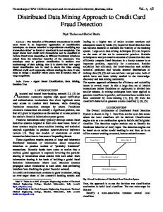
Probability 0.0 0.1 0.2 0.3 0.4 0.5 0.6 0.7 0.8 0.9 1.0
Label 0 1 0 0 1 0 1 1 0 1 1
(a) Set of probabilities and their respective class label
(b) ROC curve of the set of probabilities
Probability 0.0 0.1 0.2 0.3 0.4 0.5 0.6 0.7 0.8 0.9 1.0
Cal Probability 0 0.333 0.333 0.333 0.5 0.5 0.666 0.666 0.666 1 1
(d) Calibrated probabilities (c) Convex hull of the ROC curve
Figure 1: Estimation of calibrated probabilities using the ROC convex hull [9]. receive cross-sell offers of long-term deposits. The remainder of the paper is organized as follows. In Section 2, the methods for calibrating probabilities are explained. Afterwards, the experimental setup is given in Section 3. Here the dataset, evaluation measures and algorithms are presented. Then the results are presented in Section 4. Subsequently, the methodology is evaluated on a different dataset. Finally, conclusions of the paper are given in Section 6.
bilities are explained. First, the method proposed in [6] to adjust the probabilities based on the difference in bad rates between the training and testing datasets. Then, the method proposed in [8], in which calibrated probabilities are extracted after modifying the ROC curve using the ROC convex hull methodology, is described.
2.1 Calibration of probabilities due to a change in base rates. One of the reasons why a probability may not be calibrated is because the algorithm is trained 2 Calibration of probabilities using a dataset with a different base rate than the one When using the output of a binary classifier as a basis on the evaluation dataset. This is something common for decision making, there is a need for a probability that in machine learning since using under-sampling or overnot only separates well between positive and negative sampling is a typical method to solve problems such as examples, but that also assesses the real probability of class imbalance and cost sensitivity [10]. In order to solve this and find probabilities that are the event [3]. In this section two methods for calibrating proba- calibrated, in [5] a formula that corrects the probabilities based on the difference of the base rates is proposed.
The objective is using p = P (j = 1|x) which was estimated using a population with base rate b = P (j = 1), to find p0 = P 0 (j = 1|x) for the real population which has a base rate b0 . A solution for p0 is given as follows: (2.1)
p − pb . p0 = b0 b − bp + b0 p − bb0
Nevertheless, a strong assumption is made by taking: P 0 (x|j = 1) = P (x|j = 1) and 0 P (x|j = 0) = P (x|j = 0), meaning that there is no change in the example probability within the positive and negative subpopulations density functions. 2.2 Calibrated probabilities using ROC convex hull. In order to illustrate the ROC convex hull approach proposed in [9], let us consider the set of probabilities given in Figure 1a. Their corresponding ROC curve of that set of probabilities is shown in Figure 1b. It can be seen that this set of probabilities is not calibrated, since at 0.1 there is a positive example followed by 2 negative examples. That inconsistency is represented in the ROC curve as a non convex segment over the curve. In order to obtain a set of calibrated probabilities, first the ROC curve must be modified in order to be convex. The way to do that, is to find the convex hull [9], in order to obtain the minimal convex set containing the different points of the ROC curve. In Figure 1c, the convex hull algorithm is applied to the previously evaluated ROC curve. It is shown that the new curve is convex, and includes all the points of the previous ROC curve. Now that there is a new convex ROC curve or ROCCH, the calibrated probabilities can be extracted as shown in Figure 1d. The procedure to extract the new probabilities is to first group the probabilities according to the points in the ROCCH curve, and then make the calibrated probabilities be the slope of the ROCCH for each group.
Table 1: Cost matrix using real financial costs
Predicted Class (pi )
Fraud Legitimate
True Class (yi ) Fraud Legitimate Ca Ca Amti 0
a transaction is identified as fraud. This label was created internally in the card processing company, and can be regarded as highly accurate. In the dataset only 40,000 transactions were labelled as fraud, leading to a fraud ratio of 0.025%. From the initial attributes, an additional 260 attributes are derived using the methodology proposed in [2] and [16]. The idea behind the derived attributes consists in using a transaction aggregation strategy in order to capture consumer spending behavior in the recent past. The derivation of the attributes consists in grouping the transactions made during the last given number of hours, first by card or account number, then by transaction type, merchant group, country or other, followed by calculating the number of transactions or the total amount spent on those transactions. For the experiments, a smaller subset of transactions with a higher fraud ratio, corresponding to a specific group of transactions, is selected. This dataset contains 1,638,772 transactions and a fraud ratio of 0.21%. In this dataset, the total financial losses due to fraud are 860,448 Euros. This dataset was selected because it is the one where most frauds are being made.
3.2 Evaluation measure. In order to evaluate the classification algorithm, a cost matrix similar to the one proposed in [5] is used. The cost matrix is shown in Table 1. This matrix differentiates between the costs of the different outcomes of the classification algorithm, meaning that it differentiates between false positives and false negatives, and also the different costs of each example. Other cost matrices have been proposed for credit card fraud detection, but none differentiates 3 Experimental setup between the costs of individual transactions, see [8]. In this section, first the dataset used for the experiments Using the cost matrix it is easy to extract a cost is described. Afterwards the measure used for evalua- measure as the sum of all individual costs: tion is explained. Lastly the partitioning of the dataset m X and the algorithms used to detect fraud are shown. (3.2) yi (pi Ca + (1 − pi )Amti ) + (1 − yi )pi Ca . 3.1 Database. In this paper a dataset provided by a large European card processing company is used. The dataset consists of fraudulent and legitimate transactions made with credit and debit cards between January 2012 and June 2013. The total dataset contains 120,000,000 individual transactions, each one with 27 attributes, including a fraud label indicating whenever
i=1
This measure evaluates the sum of the cost for m transactions, where yi and pi are the real and predicted labels, respectively. 3.3 Database partitioning. From the dataset, 3 different datasets are extracted:
total train,
Table 2: Description of datasets Database Total Train Under-sampled Validation Test
Transactions 1,638,772 815,368 3,475 412,137 411,267
Frauds 0.21% 0.21% 49.93% 0.22% 0.21%
Losses 860,448 416,369 416,369 238,537 205,542
methodology can be found in [4]. Finally, two new models are evaluated by calibrating the probabilities using the methods described in Section 2, and afterwards applying BMR with the calibrated probabilities. This procedure of probability calibration is made on the validation dataset and evaluated as all other methods on the test dataset. 4
validation and test. Each one containing 50%, 25% and 25% of the transactions respectively. Afterwards, because classification algorithms suffer when the label distribution is skewed towards one of the classes [10], an under-sampling of the legitimate transactions is made, in order to have a balanced class distribution. The under-sampling has proved to be the better approach for such problems, see [10]. A new training dataset containing a balanced number of frauds and legitimate transactions is created. Table 2, summarizes the different datasets. It is important to note that the under-sampling procedure was only applied to the training dataset since the validation and test datasets must reflect the real fraud distribution. 3.4 Algorithms. For the experiments a BMR method using the probabilities of a random forest (RF) algorithm is used. The RF is trained using the undersampled and training datasets, to be able to observe the effect of different positive base rates on the probabilities and the BMR. The RF algorithm is trained using the implementation of Scikit-learn [14]. In order to have a good range of probability estimates, the parameters of the RF are tuned. Specifically, 500 not pruned decision trees with Gini criterion for measuring the quality of a split were created. As a benchmark Logistic Regression (LR) and Decision Tree (DT) are also used in conjunction with BMR. After the probability estimates are calculated, the BMR method using the cost matrix described in Table 1 is applied in order to predict whenever a transaction is legitimate or fraud. As defined in [11], the Bayes minimum risk classifier is a decision model based on quantifying tradeoffs between various decisions using probabilities and the costs that accompany such decisions. In the case of credit card fraud detection, a transaction is classified as fraud if the following condition holds true: (3.3)
Ca P (pf |x) + Ca P (pl |x) ≤ Amti P (pf |x),
and as legitimate if false. Where P (pl |x) is the estimated probability of a transaction being legitimate given x, similarly P (pf |x) is the probability of a transaction being fraud given x. Lastly, Amti is the amount of the transaction i. An extensive description of the
Results
First a RF using the under-sampled (RF-u) and the training datasets (RF-t) are calculated and then evaluated using the test dataset. Additionally to the cost measure, traditional evaluation measures such as Brier score, precision (pre), recall (rec) and F1 -Score are compared. For the calculation of the cost, the parameter Ca is estimated to be 10 Euros. This parameter has been set with the help of the card processing company internal risk team. Results are shown in Table 4. The first important thing to note, is that when using RF-u the cost is higher than the total amount lost due to fraud in the test dataset, which is 205,542 Euros. The reason for that is the low precision that translates in a high false positive rate, which is very expensive since many accounts should be analyzed before a fraud is detected. On the other hand, when using the full training dataset, a lower detection of frauds is made but with a higher precision. Nevertheless, the savings are only 8.45%, which leaves space for improvement. Also, there is a significant difference between the Brier score of both models. The reason is that by applying under-sampling the RF-u is trained using a dataset with a different base rate than the test dataset, i.e. P (pf ) 6= P 0 (pf ). This leads to having probabilities that are not calibrated, and therefore not suitable for decision making tasks [3]. In order to find a better result, the BMR model is used. This model first uses the probabilities estimated by the RF-u and the RF-t, and afterwards predicts whenever a transaction is fraud or legitimate using equation (3.3). When this methodology is used with RF-u in the performance is much worse than the RF-u, and the reason is that the probabilities of the RF-u are not calibrated. On the other hand, when the BMR is applied to the RF-t, there is an increase in the detection of frauds, while maintaining a relatively good precision. This leads to savings of 41.7%, a significant increase compared to using only the RF-t algorithm. Afterwards, in order to see how well the probabilities are calibrated, they are compared against the actual fraud rate P (pf ) for each value of the estimated probability. As can be seen on Figure 2a, the RF-u is far away from being calibrated since there is a strong difference between the predicted probability and the real fraud distribution. However, the RF-t model looks better since
(a) Comparison of the RF trained with the undersampled and full training datasets.
(b) Comparison of the calibration of probabilities methods.
Figure 2: Comparison between the estimated probability and the actual fraud rate of the different models. It is shown that the initial probabilities are neither calibrated or monotonic. On one hand, using the RF-u, there is no relation between estimated probabilities and the actual fraud rate, and also on the RF-t the relation is not monotonically increasing as expected. However, when the method for calibrating the probabilities using the ROCCH is used, the extracted probabilities are closer to the base line. In the case of the calibration method by adjusting for the difference in the base rates, the new probabilities are not as close to the base line. it is closer to the base line, which is also reflected by a lower Brier score. Nevertheless, there are some segments in which when the estimated probability is higher than actual fraud rate. Subsequently, in order to obtain calibrated probabilities the methods described in Section 2 are used. First, new probabilities are extracted by applying equation (2.1) using the under-sampled dataset (RF-u-cal br). Then, the method for calibration using the ROCCH is implemented using the probabilities of the model trained with the under-sampled dataset (RF-u-cal ROCCH) and the one with the full training dataset (RF-t-cal ROCCH). On Figure 2b, the new probabilities are shown. It can be seen that the method of calibration based on the ROCCH performs better since the probabilities RF-u-cal ROCCH and RF-t-cal ROCCH are much closer to the base line, and do not have the non-monotonic steps that the RF-u and RF-t probabilities have. This can also be seen on the ROC curves of the probabilities, since as mentioned before, non-monotonic steps in the probabilities are related to non convex segments across the ROC curve. In Figure 3a, the ROC curve of RF-u and RF-u-cal ROCCH are shown. As can be seen in detail in Figure 3b, the RF-u-cal ROCCH fixes those segments across the ROC curve that where not convex. Furthermore, as can be seen on Table 3, the impact of calibrating the probabilities of the under-sampled model is demonstrated by an important difference be-
Table 3: Brier score of the different probabilities Algorithm RF-u RF-u-cal br RF-u-cal ROCCH RF-t RF-t-cal ROCCH
Brier score 0.07957046 0.00217812 0.00189893 0.00167922 0.00167826
tween the Brier score of the RF-u and the calibrated models. However, there is neither a significant difference between RF-u-cal br and RF-u-cal ROCCH, or RF-t and RF-t-cal ROCCH. The reason for this is that the Brier score is weighted by the population, and as can be seen on Figure 4, 99.5% of the population have a probability of fraud lower than 0.05, measured using RF-t-cal ROCCH, which is expected due to the low percentage of frauds in the dataset. More interesting is that 99.5% of the losses due to fraud have a fraud probability lower than 0.15, which means that the losses do not have the same distribution as the population. Previous attempts have been made to include the cost sensitivity on the Brier score [7]. Nevertheless, they assume that the cost does not depend on the example but only on the class, which as previously explained is not the case in credit card fraud detection. Subsequently, using the calibrated probabilities estimated using the cal br and cal ROCCH methods, a BMR classifier is estimated for each one. Results of ap-
(a) ROC curve of RF-u and RF-u-cal ROCCH
(b) Zoom of the ROC curve
Figure 3: The ROC curves of the RF-u and RF-u-cal ROCCH are shown. It can be seen that for the RF-u-cal ROCCH all segments across the ROC curve that where not convex previously become convex. the probabilities. Lastly, between the two calibration methodologies, cal ROCCH-BMR arises to better results, which confirms the previously stated conclusion, since cal ROCCH-BMR is fixing the problems due to different class distributions and non-monotonicity of probabilities, but cal br-BMR only the first one. Finally, the methods are also tested using different models, in particular DT and LR. After performing the same procedure as with RF, the cost of the different algorithms is calculated. In Table 4, the results are shown. The cal ROCCH-BMR is consistently the best model measured by cost, independently of which model is used to estimate the probabilities. Nevertheless, in the case of LR, the LR-u-cal ROCCH-BMR is slightly Figure 4: Cumulative distribution of the population and better than LR-t-cal ROCCH-BMR, which may suggest the losses versus RF-t-cal ROCCH. It is show, that the that for LR it is more difficult to find a good model population does not have the same distribution as the without using under-sampling. Lastly, RF outperforms losses, which means that the losses are concentrated on both DT and LR, as it is the model whit maximum savings. higher probabilities of fraud. plying these algorithms are shown on Table 4. It can be seen that the Bayes minimum risk using the calibrated probabilities by the cal ROCCH method and the RF-t algorithm outperforms the other models measured by cost, leading to savings of 89,362 Euros or 43.5% of the losses on the test dataset. Nevertheless, the difference of results when applying cal ROCCH-BMR whit RF-t is not as significant as when the method is applied with RF-t. The reason is that the calibration method in the first case is solving both the convexity of the ROC curve and the fact that P (pf ) 6= P 0 (pf ). In the second case there is no under-sampling (P (pf ) = P 0 (pf )), which leads to the conclusion that the effect due to using different base distributions is much more important than the one due to the lack of monotonicity of
5
Evaluation on a different application
Since the contract with the card processing company, that provided the dataset for this study, forbids the publication of the database and there isn’t a publicly available credit card fraud dataset, a comparable dataset was used in order to allow reproducibility of the results and test the consistency of them across applications. In particular, a direct marketing dataset [13] available on the UCI machine learning repository [1], is used. The dataset contains 45,000 clients of a Portuguese bank who where contacted by phone between Mar 2008 and Oct 2010 and received an offer to open a longterm deposit account with attractive interest rates. The dataset contains features such as age, job, marital
Table 4: Results of the different algorithms
RF-u RF-u-BMR RF-u-cal br-BMR RF-u-cal ROCCH-BMR RF-t RF-t-BMR RF-t-cal ROCCH-BMR DT-u DT-u-BMR DT-u-cal br-BMR DT-u-cal ROCCH-BMR DT-t DT-t-BMR DT-t-cal ROCCH-BMR LR-u LR-u-BMR LR-u-cal br-BMR LR-u-cal ROCCH-BMR LR-t LR-t-BMR LR-t-cal ROCCH-BMR
Brier score 0.07957046 0.07957046 0.00217812 0.00189893 0.00167922 0.00167922 0.00167826 0.15007769 0.15007769 0.15007769 0.00203345 0.00341506 0.00341506 0.00193991 0.10437865 0.10437865 0.00519054 0.00200200 0.00203165 0.00203165 0.00197370
Table 5: Cost matrix of the direct marketing dataset
Predicted Class (pi )
Accept Decline
precision 0.0183 0.0049 0.1329 0.0851 0.7427 0.0903 0.1337 0.0112 0.0119 0.0119 0.0139 0.2183 0.2218 0.2036 0.0122 0.0050 0.0414 0.0363 0.2097 0.1090 0.1177
1 Interest rate spread is the difference between the effective lending rate and the cost of funds.
F1 −Score 0.0359 0.0098 0.1788 0.1420 0.2061 0.1516 0.2052 0.0220 0.0235 0.0235 0.0178 0.2361 0.2286 0.2139 0.0241 0.0100 0.0718 0.0632 0.0287 0.1119 0.1384
Cost 426,550 1,481,011 145,676 132,920 188,167 119,789 116,180 654,782 557,417 557,417 195,449 167,135 166,707 166,246 609,944 1,437,617 173,291 169,210 203,659 179,199 173,739
Table 6: Description of datasets of the direct marketing dataset
True Class (yi ) Accept Decline Ca Ca Inti 0
status, education, average yearly balance and current loan status and the label indicating whether or not the client accepted the offer. Similarly, as in credit card fraud the direct marketing problem is also cost sensitive, since in both there are different costs of false positives and false negatives. Specifically, in direct marketing, false positives have the cost of contacting the client, and false negatives have the cost due to the loss of income by failing to contact a client that otherwise would have opened a long-term deposit. Given the previous information, a cost matrix that collects the different costs is constructed, as shown in Table 5. Where Ca is the administrative cost of contacting the client, as is credit card fraud, and Inti is the expected income when a client opens a long-term deposit. This last term is defined as the long-term deposit amount times the interest rate spread1 . In order to estimate Inti , first the long-term deposit amount is assumed to be a 20% of the average yearly
recall 0.8804 0.8613 0.2737 0.4253 0.1197 0.4727 0.4419 0.8232 0.7427 0.7427 0.0249 0.2571 0.2258 0.2351 0.8579 0.8579 0.2712 0.2452 0.0154 0.1149 0.1682
Database Total Train Undersampled Validation Test
No Trx 47,562 19,119 4,819 11,809 11,815
Accept 12.56% 12.64% 50.17% 12.78% 12.23%
Int 394,211 156,676 42,443 97,498 97,594
balance, and lastly, the interest rate spread is estimated to be 2.463333%, which is the average between 2008 and 2010 of the retail banking sector in Portugal as reported by the Portuguese central bank. Given that, the Inti is equal to (balance ∗ 20%) ∗ 2.463333%. In a similar way as in credit card fraud, using the cost matrix a cost measure is constructed as the sum of all individual costs: (5.4)
m X
yi (pi Ca + (1 − pi )Inti ) + (1 − yi )pi Ca ,
i=1
where pi is the predicted label and yi is the ground truth. Subsequently, the dataset is split in training, under-sampling, validation and test. Relevant information of the datasets is shown on Table 6. Afterwards, the different models are calculated and evaluated. First a DT, LR and RF are calculated, using both the under-sampled and the training datasets. Next, a Bayes minimum risk decision using the cost
(a) Comparison of the RF trained with the undersampled and full training datasets.
(b) Comparison of the calibration of probabilities methods.
Figure 5: Comparison between the estimated probability and the actual fraud rate of the different models on the direct marketing dataset. It is show that the initial probabilities are not calibrated. Nevertheless, when the cal ROCCH method is used, the new probabilities look much more calibrated than the initial ones. matrix is created, and an offer is classified as accepted if the following condition holds true:
are calibrated either using cal br or cal ROCCH, better results measured by cost are found. Lastly, the best model measured by cost is the LR-u-cal ROCCH-BMR. (5.5) Ca P (pf |x) + Ca P (pl |x) ≤ Amti P (pf |x), This model arises to a cost of 5,820 Euros on the test and not accepted otherwise. Finally, the probabilities dataset, which means savings of 49.26% against the are calibrated using the methods described in Section 2, option of contacting every client. and a BMR model using the calibrated probabilities is 6 Conclusions applied. In this paper the importance of using calibrated probaOn Figure 5a, probabilities estimated with the RF bilities for the process of decision making in the context model with under-sampling and with the full training of credit card fraud detection and in general in cost sendataset are shown. It can be seen that the RF-t sitive classification has been shown. The experiments model is better calibrated than the RF-u, which as confirmed that using calibrated probabilities followed previously described, is expected since the second one by Bayes minimum risk significantly outperform using is trained with an under-sampled dataset. However, just the raw probabilities with a fixed threshold or apneither of the probabilities are well calibrated. In plying Bayes minimum risk with them, in terms of cost, order to obtain calibrated probabilities the methods false positive rate and F1 -Score. described in Section 2 are applied. On Figure 5b, it can be seen that when using the cal ROCCH on the RF-u and RF-t datasets, the probabilities are better References calibrated compared against RF-u and RF-t, and the cal br method. However, it is interesting that when [1] K. Bache and M. Lichman, UCI Machine Learning measured by the Brier score, as shown in Table 7, the Repository, School of Information and Computer Scical br method is the better one. This can be explained ence, University of California, (2013). by the fact that the population is concentrated on lower [2] Siddhartha Bhattacharyya, Sanjeev Jha, probabilities in which the cal br is well adjusted. Kurian Tharakunnel, and J. Christopher Finally, it is interesting that the best model selected Westland, Data mining for credit card fraud: A by F1 -Score is not the one that has the lower cost, comparative study, Decision Support Systems, 50 and the reason for that is that this metric is not cost (2011), pp. 602–613. sensitive and assumes a constant false negative cost, [3] Ira Cohen and Moises Goldszmidt, Properties and which as explained before is not the case in the direct Benefits of Calibrated Classifiers, in Knowledge Dismarketing problem. Overall, similar results are found covery in Databases: PKDD 2004, vol. 3202, Springer Berlin Heidelberg, 2004, pp. 125–136. as in credit card fraud, in which when the probabilities
Table 7: Results using the direct marketing dataset
RF-u RF-u-BMR RF-u-cal br-BMR RF-u-cal ROCCH-BMR RF-t RF-t-BMR RF-t-cal ROCCH-BMR DT-u DT-u-BMR DT-u-cal br-BMR DT-u-cal ROCCH-BMR DT-t DT-t-BMR DT-t-cal ROCCH-BMR LR-u LR-u-BMR LR-u-cal br-BMR LR-u-cal ROCCH-BMR LR-t LR-t-BMR LR-t-cal ROCCH-BMR
Brier score 0.22327 0.22327 0.10150 0.10541 0.10889 0.10889 0.10211 0.41138 0.41138 0.11023 0.41138 0.19995 0.19995 0.10907 0.20459 0.20459 0.09845 0.09863 0.09783 0.09783 0.09796
[4] Alejandro Correa Bahnsen, Aleksandar Stojanovic, Djamila Aouada, and Bjorn Ottersten, Cost Sensitive Credit Card Fraud Detection using Bayes Minimum Risk, in International Conference on Machine Learning and Applications, 2013. [5] Charles Elkan, The Foundations of Cost-Sensitive Learning, in Seventeenth International Joint Conference on Artificial Intelligence, 2001, pp. 973–978. [6] European Central Bank, Second report on card fraud, tech. report, 2013. [7] Peter Flach, Jose Hernandez-Orallo, and Cesar Ferri, Brier Curves : A New Cost-Based Visualisation of Classifier Performance, in International Conference on Machine Learning, 2011, pp. 1–27. [8] David J. Hand, Christopher Whitrow, Niall M. Adams, Piotr Juszczak, and David J. Weston, Performance criteria for plastic card fraud detection tools, Journal of the Operational Research Society, 59 (2007), pp. 956–962. [9] Jose Hernandez-Orallo, Peter Flach, and Cesar Ferri, A Unified View of Performance Metrics : Translating Threshold Choice into Expected Classification Loss, Journal of Machine Learning Research, 13 (2012), pp. 2813–2869. [10] Jason Van Hulse and Taghi M Khoshgoftaar, Experimental Perspectives on Learning from Imbalanced Data, in International Conference on Machine Learning, 2007. [11] Ghosh Jayanta K., Delampady Mohan, and Samanta Tapas, Bayesian Inference and Decision
precision 0.2168 0.1658 0.2001 0.2138 0.4551 0.2212 0.1950 0.1782 0.1897 0.1663 0.1897 0.2600 0.2693 0.1715 0.2385 0.1594 0.2113 0.2128 0.6641 0.2087 0.2101
[12]
[13]
[14]
[15]
[16]
recall 0.6104 0.7466 0.4624 0.4893 0.2173 0.4539 0.4492 0.6089 0.5440 0.4077 0.5435 0.3003 0.2671 0.4089 0.6016 0.7598 0.4636 0.4478 0.182 0.4636 0.4602
F1 −Score 0.3201 0.2715 0.2793 0.2974 0.2942 0.2976 0.2720 0.2756 0.2815 0.2362 0.2810 0.2786 0.2683 0.2416 0.3416 0.2637 0.2903 0.2883 0.2856 0.2878 0.2883
Cost 9,199 7,083 5,901 6,009 13,164 6,810 5,969 10,540 9,793 6,198 9,793 13,508 13,299 6,146 8,331 7,274 5,820 5,884 13,961 5,884 5,860
Theory, in An Introduction to Bayesian Analysis, vol. 13, Springer New York, Apr. 2006, pp. 26–63. Sam Maes, Karl Tuyls, Bram Vanschoenwinkel, and Bernard Manderick, Credit card fraud detection using Bayesian and neural networks, in Proceedings of NF2002, 2002. Sergio Moro, Raul Laureano, and Paulo Cortez, Using data mining for bank direct marketing: An application of the crisp-dm methodology, in European Simulation and Modelling Conference, Guimares, Portugal, 2011, pp. 117–121. F. Pedregosa, G. Varoquaux, A. Gramfort, V. Michel, B. Thirion, O. Grisel, M. Blondel, P. Prettenhofer, R. Weiss, V. Dubourg, J. Vanderplas, A. Passos, D. Cournapeau, M. Brucher, M. Perrot, and E. Duchesnay, Scikit-learn: Machine learning in Python, Journal of Machine Learning Research, 12 (2011), pp. 2825–2830. David J. Weston, David J. Hand, Niall M. Adams, Christopher Whitrow, and Piotr Juszczak, Plastic card fraud detection using peer group analysis, Advances in Data Analysis and Classification, 2 (2008), pp. 45–62. Christopher Whitrow, David J. Hand, Piotr Juszczak, David J. Weston, and Niall M. Adams, Transaction aggregation as a strategy for credit card fraud detection, Data Mining and Knowledge Discovery, 18 (2008), pp. 30–55.