Critical Line in Random Threshold Networks with Inhomogeneous ...

Critical Line in Random Threshold Networks with Inhomogeneous Thresholds Thimo Rohlf

arXiv:0707.3621v2 [cond-mat.dis-nn] 21 Feb 2008

Santa Fe Institute, 1399 Hyde Park Road, Santa Fe, NM 87501, U.S.A (Dated: February 21, 2008) We calculate analytically the critical connectivity Kc of Random Threshold Networks (RTN) for homogeneous and inhomogeneous thresholds, and confirm the results by numerical simulations. We find a super-linear increase of Kc with the (average) absolute threshold |h|, which approaches Kc (|h|) ∼ h2 /(2 ln |h|) for large |h|, and show that this asymptotic scaling is universal for RTN with Poissonian distributed connectivity and threshold distributions with a variance that grows slower than h2 . Interestingly, we find that inhomogeneous distribution of thresholds leads to increased propagation of perturbations for sparsely connected networks, while for densely connected networks damage is reduced; the cross-over point yields a novel, characteristic connectivity Kd , that has no counterpart in Boolean networks. Last, local correlations between node thresholds and in-degree are introduced. Here, numerical simulations show that even weak (anti-)correlations can lead to a transition from ordered to chaotic dynamics, and vice versa. It is shown that the naive meanfield assumption typical for the annealed approximation leads to false predictions in this case, since correlations between thresholds and out-degree that emerge as a side-effect strongly modify damage propagation behavior. PACS numbers: 05.45.-a, 05.65.+b, 89.75.-k, 89.75.Da

I.

INTRODUCTION

Many systems in nature, technology and society can be described as complex networks with some flow of matter, energy or information between the entities the system is composed of; examples are neural networks, gene regulatory networks, food webs, power grids and friendship networks. Often, in particular when the networks considered are very large, many details of the topological structure as well as of the dynamical interactions between units are unknown, hence, statistical methods have to be applied to gain insight into the global properties of these systems. In this spirit, Kauffman [1, 2] introduced the notion of Random Boolean Networks (RBN), originally as a simplified model of gene regulatory networks (GRN). In a RBN of size N , each node i receives inputs from 0 ≤ k ≤ N other nodes (with k usually either considered to be constant, or distributed accord¯ ≪ N ), and updates ing to a Poissonian with average K its state according to a Boolean function fi of its inputs; the subscript i indicates that Boolean functions vary from site to site, usually assigned at random to each node. It was shown that RBN exhibit a percolation transition from ordered to chaotic dynamics at a critical ¯ = Kc = 2. Since interactions in RBN connectivity K are asymmetric and hence a Hamiltonian does not exist, mean-field techniques have to be applied for analytical calculation of critical points, for example the so-called annealed approximation (annealed approximation) introduced by Derrida and Pomeau [3, 5, 6]. In the annealed approximation, random perturbations are applied to initial dynamical states, and random ensemble techniques are applied to determine whether the so-induced ”damage” spreads over the network or not. Recent research has revealed many surprising details of RBN dynamics at criticality, e.g. super-polynomial scaling of the number

of different dynamical attractors (fixed points or periodic cycles) √ with N [7] (while Kauffman assumed it to scale ∼ N [1]), as well as analytically derived scaling laws for mean attractor periods [8] and for the number of frozen and relevant nodes in RBN [9, 10]. Similarly, it was shown recently that dynamics in finite RBN exhibits considerable deviations from the annealed approximation (that is exact only in the limit N → ∞) [11, 12]. Boolean network models have been applied successfully to model the dynamics of real biological systems, e.g. the segment polarity network of Drosophila [13], dynamics and robustness of the yeast cell cycle network [14], damage spreading in knock-out experiments [15] as well as establishment of position information [16] and cell differentiation [17] in development. Other models explicitly evolve RBN topology according to local rewiring rules coupled to local order parameters of network dynamics (e.g., the local rate of state changes), and investigate the resulting self-organized critical state [18, 19, 20]. A drawback of RBN is the fact that, in spite of their discrete nature (which makes them easy to simulate on the computer in principle), the time needed to compute their dynamics in many instances scales exponential in N ¯ and often large statistical ensembles are needed and K, for unbiased statistics due to the strongly non-ergodic character [21] of RBN dynamics. For this reason, there exists considerable interest in simplified models of RBN dynamics, as, for example, Random Threshold Networks (RTN), that constitute a subset of RBN. In RTN, states of network nodes are updated according to a weighted sum of their inputs plus a threshold h, while interaction weights take (often discrete and binary) positive or negative values assigned at random. The critical connectivity, calculated by means of the annealed approximation, was found to deviate slightly from RBN [22, 23, 24]; this analysis was extended to RTN dynamics

2 including stochastic update errors [25]. In particular, it was found that phase transitions in RTN with scale-free topologies [25, 26] substantially differ from both RTN with homogeneous or Poissonian distributed connectivity and scale-free RBN [27]. Further, dynamics in finite RTN with k = const. = 2 inputs per node recently was found to be surprisingly ordered, including, e.g., globally synchronized oscillations [28]. Other approaches, that apply learning algorithms as well as ensemble techniques, present evidence that information processing of static [29] or time-variant [30] external inputs is optimized at criticality in both RBN and RTN. In this paper, we extend the theoretical analysis of RTN in a number of respects. First, we calculate the critical connectivity Kc for arbitrary thresholds h ≤ 0, and generalize this derivation for the first time to inhomogeneously distributed thresholds hi that can vary from node to node. This generalization, that introduces an additional level of complexity to RTN dynamics, is motivated by recent observations of strong variations in regulatory dynamics from gene to gene in real GRN, caused by, for example, the frequent occurrence of canalizing functions [21] and the abundance of regulatory RNA in multicellular organisms which strongly influence the expression levels and -patterns of (regulatory) proteins [31]. Using the annealed approximation and additional approximation techniques, we derive a general scaling relationship between critical connectivity Kc and (average) absolute node threshold |h|, and show that Kc (|h|) asymptotically approaches a unique scaling law Kc (|h|) ∼ h2 /(2 ln |h|) for large |h|. Evidence is presented that this asymptotic scaling law is universal for RTN with Poissonian distributed connectivity and threshold distributions with a variance that grows slower than |h|2 . Convergence against this scaling law is rather slow (logarithmic in |h|); we show that, for finite |h|, scaling behavior can be approximated well locally by power laws Kc (|h|) ∼ |h|α with 3/2 < α < 2. Further, we establish that damage propagation functions of RTN with homogeneous thresholds |h| and of RTN with inhomogeneous thresholds with the same av¯ = |h| intersect at characteristic connectivities erage |h| ¯ < Kd , ranKd (|h|) > Kc (|h|), which implies that for K dom distribution of thresholds tends to increase damage, ¯ > Kd , the opposite holds. Evidence is prewhile for K sented that Kd (|h|) converges to an asymptotic scaling law Kd (|h|) ∼ h2 . We compare the scaling of Kd to the corresponding case of random Boolean networks (RBN) with inhomogeneously distributed bias, parameterized in terms of a bias parameter 1/2 ≤ p ≤ 1. It is shown that Kd is not defined for RBN in the limit p → 1, which corresponds to |h| → ∞ in RTN. Hence, Kd constitutes a truly novel, not previously known concept, yielding a new characteristic connectivity which is well-defined only for RTN. Last, we investigate the effect of correlations between thresholds hi and in-degree ki , while keeping all other network parameters constant. We find that even small

positive correlations can induce a transition from supercritical (chaotic) to subcritical (ordered) dynamics, while anti-correlations have the opposite effect. It is shown that the naive mean-field assumption typical for the annealed approximation leads to false predictions in this case. Even in the simplest case, where only in-degree and (absolute) threshold are correlated, complete information about topology, including the output side, has to enter statistics, and the order of averages becomes important.

II.

RANDOM THRESHOLD NETWORKS

A Random Threshold Network (RTN) consists of N randomly interconnected binary sites (spins) with states σi = ±1. For each site i, its state at time t+1 is a function of the inputs it receives from other spins at time t: σi (t + 1) = sgn (fi (t))

(1)

with fi (t) =

N X

cij σj (t) + hi ,

(2)

j=1

where cij are the interaction weights. If i does not receive signals from j, one has cij = 0, otherwise, interaction weights take discrete values cij = ±1, +1 or −1 with equal probability. In the following discussion we assume that the threshold parameter takes integer values hi ≤ 0 [34]. Further, we define sgn(0) = −1. [35] The N network sites are updated synchronously. Notice that we depart from the well-studied case hi = const. = 0 in two respects: hi can take arbitrary values hi ≤ 0, and it can differ from node to node (inhomogeneous thresholds). Let us now have a closer look on network topology. Let ¯ be the average connectivity, i.e. the average number K of inputs (outputs) per site, and let us assume that each ¯ interaction weight has equal probability p = K/N to take a non-zero value. Further, let us consider the limit ¯ ≪ N . Under of sparsely connected networks with K these assumptions, the statistical distribution ρk of inand out-degrees follows a Poissonian:

ρk =

¯k K ¯ e −K . k!

(3)

Further, we study the case where in- and out-degree distributions differ: while the out-degree is still distributed according to a Poissonian, the in-degree distribution exhibits a power-law tail, i.e. ρkin ∝ k −γ with 2 ≤ γ ≤ 4.

(4)

3

1

CALCULATING THE CRITICAL LINE A.

Uniform threshold h < 0

0.8

We start with the simplest case and assume that all network sites have identical integer threshold values hi ≡ h ≤ 0. The case h > 0 is not studied here, as it may lead to the pathological outcome of nodes set to an active state σi = +1, though they receive only inhibitory inputs cij < 0. Let us first calculate the probability for damage spreading ps (k), i.e. the probability that a node with k inputs changes its state, if one of its input states is flipped. A straight-forward extension of the combinatorial analysis carried out in [24] for the special case h = 0 yields    k ps (k, |h|) = k −1 · 2−(k+1) · (k + |h| + 1) · k+|h|+1 2   k (5) +(k − |h| + 1) · k−|h|+1 2

= 2−(k−1)



(k − 1)



|h|=0 |h|=2 |h|=3 |h|=5 |h|=10 asymptotic decay

ps (k, |h|)

III.

0.6 0.4 0.2 0

1

FIG. 1: Probability ps (k, |h|) of damage propagation, for different values of the threshold |h|, as a function of the number of inputs √ k. For large k, the curves asymptotically approach ps ∼ 1/ k (dashed line). Notice the oscillatory behavior for |h| > 0.

for odd k − |h| with k > |h|, and    k ps (k, |h|) = k −1 · 2−(k+1) · (k − |h|) · k−|h|  2  k (7) +(k + |h| + 2) · k+|h|+2

2

2

= 2

k+|h| 2

(8)

for even k − |h| with k > |h| (for a detailed derivation, please refer to appendix A). Notice that Eqs. (6) and (8) are similar, yet not identical to the corresponding relations derived in [25] for RTN with probabilistic time evolution; in particular, for the RTN with deterministic dynamics as studied here, the relation podd s (k) = ps (k−1) holds only for the special case |h| = 0, whereas for |h| > 0, ps (k) exhibits an oscillatory behavior (Fig. 1). If we know the statistical distribution function ρk of the in-degree, the average damage spreading probability then simply follows as [24] hps i =

N X

k=|h|

ρk ps (k + 1, |h|),

(9)

where h.i indicates the average over the ensemble of all possible network topologies that can be generated according to the degree-distribution ρk . In the case of a Poisson ¯ it distributed connectivity with average degree degree K, follows ¯ |h|) = e−K¯ hps i(K,

N X

k=|h|

¯k K ps (k + 1, |h|). k!

(10)

d(K)

2.5

  −(k−1) (k − 1)

100

k

(6)

k+|h|−1 2

10

1.5 1 0.5 0

0

1

2

3

4

5

6

7

8

9

10

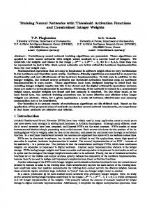
K FIG. 2: Expectation value d¯ of damage one time step after a one-bit perturbation, as a function of the average connectivity ¯ and different (homogeneous) thresholds |h| (|h| = 0 (+), K, |h| = 1 (X), |h| = 2 (*), |h| = 3 (), |h| = 4 (♦). Solid curves are the corresponding analytical results obtained from the annealed approximation.

Let us now apply the so-called annealed approximation [3], which averages the effect of perturbations over the whole ensemble of possible network topologies and all possible state configurations; in this approximation, the expected damage d¯ after one update time step, given a one-bit perturbation at time t − 1 then follows as ¯ + 1) = hps i(K, ¯ |h|) · K, ¯ d(t

(11)

where ¯. denotes the average over all possible network topologies and all possible state configurations. If we

2.5

2.5

2

2

1.5

1.5

|h|=3

1

1

0.5

0.5

0

|h|=1 |h|=2

d(K)

d(K)

4

0

0

1

2

3

4

5

6

7

8

9

10

|h|=4

0

apply a sufficiently large (but finite) upper limit N to the sum in Eq. (10), we can numerically evaluate this formula with any desired accuracy. Figure 2 shows the results for the first five values of negative h of RTN with Poissonian distributed connectivity, compared to measurements obtained from numerical simulations of large ensembles of randomly generated instances of RTN, indicating an excellent match between theory and simulation. B.

Poisson distributed thresholds

Let us now consider the more general case of nonuniform thresholds, i.e., networks where each site i has assigned an individual threshold hi ≤ 0. In the simplest case, we can imagine that the final thresholds resulted from iterated, random decrementations (starting from h = 0 for all sites), until a certain average threshold ¯ is reached - this process results in Poisson distributed h thresholds hi . If threshold assignment is independent from the (also Poisson distributed) in-degree, the probabilities for k and h simply multiply, and the resulting average damage propagation probability is ¯ ¯ |h|) ¯ = e−(K+ ¯ |h|) hps i(K,

N N ¯ |h| X X ¯ k |h| K ps (k + 1, |h|), k!|h|!

|h|=0 k=|h|

(12)

¯ is the average absolute threshold. where |h| Figure 3 demonstrates that the expected damage

2

3

4

5

6

7

8

9

10

K

K ¯ K) ¯ one time step after a one-bit FIG. 3: Average damage d( perturbation, for Poisson-distributed connectivity with aver¯ and Poisson-distributed negative thresholds age degree K, ¯ points are data from numerwith average absolute value |h|; ical simulations of RTN (ensemble averages over 100000 different network realizations for each data point), lined curves are analytical solutions (annealed approximation). Numerical ¯ = 0 (+), |h| ¯ = 0.3 (X), |h| ¯ = 1.0 data where sampled for |h| ¯ = 1.5 (squares), |h| ¯ = 2.5 (⋄), |h| ¯ = 3.5 (triangle) and (*), |h| ¯ = 5.0 (+). |h|

1

FIG. 4: Comparison of damage spreading in networks with homogenenous thresholds |h| = const. (solid lines, threshold values |h| as indicated) vs. networks with inhomogeneous thresholds distributed according to a Poissonian with the ¯ (curves with data points, |h| ¯ =1 same average threshold |h| ¯ ¯ ¯ (+), |h| = 2 (x), |h| = 3 (*) and |h| = 4 (); results obtained from the annealed approximation.

¯ resulting from a one-bit perturbation at time ¯ |h|) d¯t+1 (K, t, as predicted from this annealed approximation over both degree- and threshold distribution, exhibits excellent agreement with the results obtained from numerical simulations of randomly generated RTN ensembles. It is an interesting question how the dynamics of RTN with inhomogeneous thresholds compares to RTN with ¯ K) ¯ for RTN homogeneous thresholds. Figure 4 shows d( with different homogeneous |h| = const. and the corresponding inhomogeneous RTN with Poisson-distributed ¯ = |h|, as obtained thresholds with the same average |h| from the annealed approximation. One observes that for ¯ the curves for RTN with inhomogeneously dissmall K, tributed thresholds are systematically above those of the corresponding homogeneous RTN, i.e., the randomization of node thresholds increases dynamical disorder also, the critical connectivities Kc (|h|) (intersections with the line d¯ = 1) are shifted to smaller values. However, one also realizes that the curves intersect in the supercritical phase at characteristic connectivities Kd (|h|), i.e., ¯ > Kd (|h|), inhomogeneity in thresholds actually for K reduces damage. C.

Universal scaling of the critical line

If we again assume a one-bit perturbation at time t, the critical line Kc (|h|), that separates the ordered and the chaotic phase of RTN dynamics, is given by the condition ¯ + 1) = hps i(Kc (|h|), |h|) · Kc (|h|) = 1. d(t

(13)

Again, we can apply Eq. (10) to solve this equation for arbitrary h ≤ 0, however, numerical evaluation is almost

5 5

the damage:

ln[d(K,|h|)]

0

¯ K, ¯ |h|)] ≈ ln [d(

−5

with C = ln −15

"

¯ −K ¯ · ln 1 − ln K  ¯ K + |h| +C ¯ − |h| K



 p 2/π ; solving this equation for ¯ c (|h|), |h|] = 0 ln [d(K

10

100

1000

K ¯ K)], ¯ as calcuFIG. 5: Logarithm of the average damage, ln [d( lated from the annealed approximation, for different values of |h| (|h| = 10 (+), |h| = 20 (X), |h| = 40 (*) and |h| = 60 ()). The corresponding solid curves are obtained from Eq. (14). ¯ one finds that Eq. (14) approximates the For not to small K, true damage function very well. 1e+07 1e+06

2 # (14)

(15)

(16)

or, more accurately, we have to find the minimum of the absolute value |∆ps /∆k| of the ’discrete derivative’ of ps (k, |h|) for even k−|h|, with ∆k = const. = 2. Inserting Eq. (8) then yields

10000 1000 100 10 1

|h| ¯ K

then yields the critical connectivity Kc (|h|). Figure 5 shows that this approximation is very accurate even for considerably small, finite |h|. In particular, one can show that for |h| ≥ 10 the relative error ǫ between the approximation of Eq. (15) and the result obtained from the annealed approximation vanishes ∼ |h|−1 (Fig. 7 ). Still, Eq. (15) has to be solved numerically to calculate Kc (|h|), and hence does not yield information about the scaling behavior in the limit |h| → ∞. A first insight into the expected scaling can be obtained from an analysis of the scaling behavior of the maximum of ps (k, |h|) with respect to |h|; if we restrict our analysis to even k − |h|, kmax is given by the condition ∆ps = ps (k, |h|) − ps (k − 2, |h|), ≈ 0

100000

Kc



− |h| ln

−10

−20

1 2

1

10

100

1000

10000

|h| FIG. 6: Scaling behavior of the critical connectivity Kc (|h|) as a function of the (homogeneous) node threshold |h|, log-logplot. Data points + are solutions obtained from the annealed approximation of Eq. (13), the solid curve is obtained from setting Eq. (14) to zero. The dashed line shows the asymptotic scaling behavior stated in Eq. ().

(k − 3)! ∆ps = 2−k+3 ·(17) [(k + |h| − 3)/2]![(k − |h| − 3)/2]!   (k − 1)(k − 2) · −1 . (k + |h| + 1)(k − |h| − 1) Obviously, the pre-factor on the right hand-side is always positive; consequently, in order to determine the maximum of ps (k, |h|), we have to solve the equation (k − 1)(k − 2) − 1 = 0. (k + |h| + 1)(k − |h| − 1) Using simple algebra, one can show that kmax = |h|2 + 1

impossible for |h| > 80 due to exponentially diverging computing time caused by evaluation of the sum in Eq. ¯ [36]. For estimation of the scaling behav(13) for large K ior of Kc (|h|) for larger |h|, we are interested in a good approximation that does not require summation over the whole network topology, and hence neglect the variation in k, considering damage propagation in the mean field ¯ (for details, see Appendix B). Uslimit k = const. ≈ K √ ing the Stirling approximation: n! ≈ nn e−n 2πn, this leads to the following approximation for the logarithm of

(18)

(19)

solves this equation, i.e. the maximum of ps (k, |h|) scales quadratically with |h|. Since ps (k, |h|) for |h| ≫ 0 vanishes both for small and large k, it is plausible that the scaling behavior of Kc is dominated by the leading behavior of the maximum of the distribution, i.e. should scale ∼ f (|h|)|h|2 , where contributions from the tails of the distribution are considered in f (|h|). A more detailed analysis carried out in appendix C ¯ and |h|, according takes into account that, for large K to the central limit theorem the Binomial distribution

6 1

ε

~1/ ln|h| ~1/|h|

0.1

ε1 (|h|) ε2 (|h|) 0.01

1

10

100

1000

10000

of the critical connectivity Kc . Figure 6 demonstrates the convergence of the critical line (straight-lined curve and data points) against this asymptote (dashed curve). For finite |h|, we notice that there are substantial contributions from additional terms that vanish only logarithmically, and hence an approximation based on Eq. (21) would substantially underestimate Kc . This can be appreciated clearly from Fig. 7, which demonstrates the slow (logarithmic) convergence of the error ε2 (|h|) made by application of Eq. (21) for finite |h|. From Fig. 6, it is also evident that, for finite |h|, Eq. (21) overestimates the slope dKc /d|h|. One can show that, for finite |h|, Kc (|h|) is better approximated locally by power-laws of the form

|h|

Kc (|h|) ≈ a(|h|) · |h|α(|h|)

FIG. 7: Crosses (X): Relative error ε1 between the approximation of Eq. (14) and the result obtained from the annealed approximation, as a function of |h|. For |h| ≥ 15, ε1 vanishes ∝ |h|−1 ; straight line with slope −1 shown for comparison. Data points (+): Relative error ε2 between the approximation of Eq. (14) and the asymptotic scaling of Eq. (21); ε2 goes to zero logarithmically (compare to dashed curve). 1.95 1.9

with 3/2 < α < 2. We confirmed this intuition by numerically inserting candidate solutions with fixed α into Eq. (14), and solving for the values of |h| and a where the deviation from the true curve Kc (|h|) becomes minimal; inverting this relation, we obtain the optimal power law exponents α(|h|) as a function of |h| (Fig. 8, for details, see appendix E). Again, we can apply the Gaussian approximation for the damage propagation function to derive upper (lower) bounds for the finite size scaling of α(|h|) and a(|h|), which yield (cf. appendix E)

1.85

α(|h|) ≈ 2 − 0.8

1.75 1.7

0.4

a(|h|) ≈

0.2 1.65

0

1.6 1.55

10

1000 100000 1e+07

|h| 10

100

1000 10000 100000 1e+06 1e+07 1e+08

|h| FIG. 8: Optimal exponents α of power-laws Kc ≈ a|h|α that approximate the scaling function Kc (|h|), as shown in Fig. 6, as a function of |h|. The dashed curves are the corresponding asymptotic estimates of Eq. (23) and Eq. (24).

that characterizes the damage propagation function Eq. (8) can be replaced by a Gaussian, consequently, the expected damage is approximated very well by r   1 h2 ¯ K, ¯ |h|) = K ¯· d( (20) exp − ¯ ¯ . 2π K 2K Taking logarithms and inserting into Eq. (15) then yields the asymptotic scaling lim Kc (|h|) =

|h|→∞

1 . ln |h|

(23)

and

0.6

a

α

1.8

(22)

h2 2 ln |h|

(21)

e . 2 ln |h|

(24)

Figure 8 shows that the true optimal values are systematically below (α) or above (a) these curves, demonstrating the non-trivial scaling behavior of the critical line for finite |h|, which is significantly different from the simple asymptotic behavior in the thermodynamic limit (Eq. (21)). Let us now investigate the scaling behavior of Kc for networks with inhomogeneous thresholds. Figure 9 shows that, for finite |h|, the critical line Kc (|h|) for RTN with inhomogeneous thresholds is always below the corresponding values for homogeneous |h|; the absolute differ¯ = |h|)| between both ence ∆Kc (|h| := |Kch (|h|) − Kci (|h| curves, however, increases only linearly in with |h| (inset of Fig. 9 ), where Kch (|h|) is the critical connectivity for ¯ the corresponding value for homogeneous |h|, and Kci (|h|) ¯ = |h|. inhomogeneously distributed |h| with mean |h| Intuitively, this is straight-forward to understand: since we assumed that k and |h| are statistically independent, ∆Kc (|h|) is determined solely by the variance σh2 of the threshold distribution around the mean threshold ¯ = |h| - the smaller this variance is, the more peaked |h| ¯ = |h|, and the less it hence this distribution is around |h| differs from the homogeneous distribution. Since we assumed that (in the inhomogeneous case) thresholds are

7 ¯ we directly conclude Poisson distributed around |h|, (25)

For arbitrary threshold distributions that are statistically independent from the networks’ degree distribution with variance σk2 , we make the ansatz 2 σtot = σk2 + σh2

800

100 10

600 500

1

0.1

400

1

¯2 h ¯ , 2 ln |h|

(28)

as it is shown in appendix C. This means that in all these ¯ → ∞ is dominated cases, the asymptotic scaling for |h| by by the scaling behavior of the maximum of the damage propagation function ps (k, |h|), with an exponent α = 2.

100 0

0

10

K (|h|) 40 linear fit

Kc(|h|)

600

∆Kc

60

20

500

0

300 200

20

40

|h|

0

40

50

60

70

¯ for networks with threshold distribuFIG. 10: Kc (β, |h|) tions following discretized Gaussian distributions with differ¯ β (for details, see text). One ent variances V ar(|h|) = |h| clearly appreciates that the larger the variance of the thresh¯ are below the old distribution, the more the curves Kc (β, |h|) critical line of networks with homogeneous thresholds (blue solid line); in the limiting case β = 1.95 ≈ α (yellow trian¯ Inset: differences gles), Kc scales almost linearly with |h|. ¯ |∆Kc (β, |h|)| to the critical line of RTN with homogeneous ¯ βe with β < βe < α (power law fits and thresholds scale ∼ |h| dashed line with slope α shown for comparsion); this implies asymptotic convergence to the universal scaling function Eq. ¯ → ∞ for all cases shown here. (28) in the limit |h| β 0.5 1.0 1.2 1.5 1.8 1.95

βe 0.533 ± 0.009 1.099 ± 0.004 1.327 ± 0.004 1.732 ± 0.004 1.942 ± 0.003 1.975 ± 0.004

60

100 0

30

TABLE I: Scaling exponents βe , as obtained from fits of ¯ βe , as a function of β. ∆Kc ∼ |h|

0

400

20

|h|

asymptotic scaling homogeneous |h| Poisson distributed |h|

700

100

200

1000 800

10

|h|

(27)

for networks with inhomogeneous thresholds distributed ¯ (for details, cf. around an average absolute threshold |h| ¯ → ∞, all appendix C). This implies that, in the limit |h| networks with Poissonian distributed connectivity and threshold distributions with a variance which obeys the ¯ β with 0 ≤ β < 2, follow the scaling relation: σh2 ∼ |h| universal asymptotic scaling relation

900

asymptotic scaling β = 0.5 β = 1.0 β = 1.2 β = 1.5 β = 1.8 β = 1.95

β =0.5 β =1.0 β =1.2 β =1.5 β=1.8 β=1.95

300

2 for the total variance σtot . Using the same Gaussian approximation as above for the homogeneous case, one can show that

¯ = Kc (|h|)

1000

700

(26)

¯2 2 ¯ ≈ h Kc (|h|) ¯ − σh 2 ln |h|

900

∆ Kc (|h|)

¯ = |h|.

Kc (|h|)

∆Kc (|h|) ∼

σh2

1000

10

20

30

40

50

60

70

Let us now confirm this finding for a different class of threshold distributions. Since in a Poissonian the variance is not a free parameter, we now instead choose a discretized Gaussian distribution, i.e.

|h| FIG. 9: Kc (|h|) for homogeneous thresholds (+) and Poisson ¯ (X), annealed distributed thresholds with the same average |h| approximation. The solid line is the asymptotic scaling obtained from Eq. (15). For inhomogeneous |h|, the critical line is systematically below Kc of networks with homogeneous |h|. Inset: The difference |∆Kc (|h|)| between both curves grows only linearly in |h|, confirming that the asymptotic scaling in the limit |h| → ∞, is the same in both cases.

P (|h|) =

1 Z ¯ 2 2 √ e− 2 (|h|−|h|) /σh σh 2π

(29)

with Z= and variance

−1  2

 m  |h| X 

1 1 ¯ 2 √ e− 2 (|h|−|h|) /σh  σ 2π |h|=0 h

¯ β, σh2 = |h|

β ∈ [0, α).

(30)

(31)

8

βe

¯ . ∆Kc ∝ |h|

¯ = |h|) Kc (β, |h| = h Kc (|h|) |h|→∞

1000

100

2

10

h − |h|

(32)

Table 1 compares β and βe (as obtained from fits of ∆Kc ; in all cases, we have βe > β, which is a discretization effect, but still βe < α. Hence, it follows that lim

10000

Kd

The factor Z ensures that the probabilities are normalized in the interval [0, |h|m ], where |h|m denotes the cutoff of the threshold distribution. Figure 10 compares the ¯ for different values of β to the scaling functions Kc (|h|) asymptotic case of homogeneous networks. Obviously, ¯ increased variance of the threshold distrifor finite |h|, bution substantially lowers the critical connectivity; in ¯ the limiting case β ≈ α, Kc grows only linearly with |h|. For β < α, we find that the deviation from the scaling behavior of RTN with homogeneous thresholds scales as

Kch (|h|) − ∆Kc (β, |h|) Kch (|h|) |h|→∞ lim

= 1 − const. · lim |h|βe −α (33)

1

1

10

100

|h| FIG. 11: Scaling behavior of Kd (|h|) as a function of |h|, double logarithmic plot. The dashed line highlights the asymptotic scaling (Eq. (36)).

|h|→∞

= 1 ¯ for βe < α, i.e. in this case all scaling functions Kc (β, |h|) for |h| → ∞ indeed asymptotically converge to the same universal scaling function, as given by Eq. (28). Let us now have a closer look at the scaling behavior of the intersection points Kd (|h|), as introduced in ¯ |h|) be the the last paragraph of subsection B. Let d¯h (K, expected damage in networks with homogeneous thresh¯ the expected damage in networks with ¯ |h|) old, and d¯i (K, inhomogeneous thresholds; then ¯ = 0 d¯h (Kd (|h|), |h|) − d¯i (Kd (|h|), |h|) ¯ = |h| |h|

(34) (35)

are the defining equations for Kd (|h|). Notice that for ¯ < Kd , the randomness introduced by inhomogeneous K thresholds actually increases the probability for damage ¯ > Kd , it is decreased. Equation spreading, whereas for K (34), under condition Eq. (35), can be solved numerically for not to large |h|. Further, one can derive the asymptotic scaling in the thermodynamic limit by application of the Gaussian approximation for the damage propagation function (for details, cf. appendix D), showing that lim Kd (|h|) = h2 − |h|.

|h|→∞

(36)

Fig. 11 demonstrates that Kd (|h|) approaches this asymptotic scaling already for considerably small |h|, indicating that Kd (|h|) is characterized by the same universal scaling exponent α = 2 as Kc (|h|). Notice, however, that the asymptotic scaling law for Kd obeys a purely algebraic relation, whereas Kc has a dependence ∼ h2 / ln |h| (Eq. 21). Let us briefly compare the scaling behavior of RTN with non-zero thresholds, as discussed above, to Random Boolean Networks (RBN). Obviously, increasing |h|

biases the output states of network nodes (for the systems discussed in this paper, it increases the probability to have an output state σi = −1). Biased RBN obey the scaling relationship [4] Kc =

1 . 2p(1 − p)

(37)

To compare this relationship to the asymptotic scaling for RTN in the limit of large |h|, we have to consider the limit p → 1. One can show that, in this limit, the scaling function Eq. (37) logarithmically approaches the asymptotic scaling Kc ≈ −

p2 . 2 ln p

(38)

This shows that |h| plays the same role as the bias parameter p in RBN, and that both classes obey the same scaling in the limit p → 1 and |h| → ∞, respectively. However, there are also substantial differences between both classes of systems, that come into play when |h| is small (when p is close to 1/2). In particular, while RBN in this limit still obey the simple scaling relationship Eq. (37)), the critical connectivity Kc of RTN is derived from the complex dependence of Eq. (14). This difference is due to the fact that, in RTN, local damage propagation strongly depends on the in-degree of nodes (cf. Eq. 6 and 8), while it is independent from the in-degree in RBN for k > 0. In the limit of sparsely connected networks (i.e. small |h| and Kc ), this leads to much stronger finite size effects in RTN than in RBN. Furthermore, in this limit also the absolute values of Kc in RTN are considerably below those of RBN [24, 25]. Finally, let us remark on the existence of the characteristic connectivity Kd . As shown above, Kd is defined for RTN with arbitrary |h|, in particular, it exists in the limit

9 |h| → ∞, with a well-defined asymptotic scaling. For biased RBN, the corresponding limit is given by p → 1 (or, equivalently, p → 0). Obviously, we can in principle assign variable (inhomogeneous) biases pi to different RBN nodes such that the average bias is equal to p. However, because p is a probability and hence 0 ≤ p ≤ 1, the variance σp2 has to vanish in the limit p → 1 (p → 0) to yield a proper average bias. Since Kd is defined by comparing networks with diverging variance of the order parameter |h| (or p, respectively) with the corresponding networks with vanishing variance and the same average |h| (or p, respectively), this implies that Kd is not defined for RBN in the limit of large bias p → 1, which corresponds to |h| → ∞ in RTN. Hence, Kd constitutes a truly novel, not previously known concept, yielding a new characteristic connectivity which is well-defined only for RTN. It is interesting to notice that the dependence of Kc , as well as of Kd on |h| is clearly super-linear even for considerably small |h|; this has profound consequences for algorithms that evolve RTN towards (self-organized) criticality by local adaptations of both thresholds and the number of inputs a node receives from other nodes [32]. In particular, it can be shown that co-evolution of network dynamics and thresholds/in-degrees leads to strong correlations between |h| and k. To approach this type of problem analytically, we will now extend our analysis in this direction. first, In the next section, we will show that even weak correlations between k and |h| can lead to a transition from sub-critical to super-critical dynamics (and vice versa), while keeping the average connectivity ¯ constant. ¯ and the average absolute threshold |h| K

ρ

0

2

4

6

8

10 12 14

j

0

2

4

6

8

|h|

10 12 14

j

i

0.1 0.08 0.06 0.04 0.02 0

=0

|h|

Generation of correlations:

i

14 12 10 8 6 4 c 2 k 0 in

0

2

4

6

8

10 12 14

14 12 10 8 c= 6 4 2 k in 0

0.2

14 12 10 8 c= 6 4 2 k 0 in

0.9

|h| after

before

Generation of anti−correlations:

i

j

i

j

FIG. 12: Schematic illustration of the algorithm applied to generate local (anti-)correlations between in-degree kin and (absolute) threshold |h|. Arrows symbolize inputs from other nodes, boxes symbolize node thresholds (one box corresponds to |h| = 1, two boxes to |h| = 2, and so on). For details of the algorithm, please refer to the text.

FIG. 13: Combined density ρ(kin , |h|) for three different positive values of the correlation parameter c, from top to bottom: c = 0, c = 0.2 and c = 0.9. Dark gray indicates a high probability density. The diagonal structure of ρ(kin , |h|) for c = 0.9 (lower panel) indicates emergence of strong positive correlations between kin and |h|.

D.

Effect of correlations between k and h

So far, we assumed that node degree and node thresholds are totally uncorrelated; while this matches well the ”maximum disorder” assumption used in random ensemble based approaches as, e.g., the annealed approximation, this might be a quite unrealistic constraint for many

10

0

2

4

6

8

10 12 14

14 12 10 8 6 4 c 2 k 0 in

1.2

0.1 0.08 0.06 0.04 0.02 0

=0

0

2

2

4

4

6

6

8

|h|

8

1.1 1.05 1 0.95 0.9 0.85

|h|

0

1.15

d

ρ

0

0.2

0.4

0.6

0.8

1

|c|

10 12 14

10 12 14

14 12 10 8 c= 6 4 2 k in 0

14 12 10 8 c= 6 4 2 k 0 in

−0.1

¯ as a function of |c|, for correFIG. 15: Average damage d(c) lated kin and |h| (+) and anti-correlated kin and |h| (X), with ¯ = 6.15 for c ≥ 0 networks, K ¯ = 5.8 for c ≤ 0 networks and K ¯ = 2.5 in both cases. Numerical data where obtained from |h| ensemble averages over Z = 5 · 105 randomly generated RTN with N = 1024 nodes for each data point. Solid curves are the corresponding results of the corrected annealed approximation, while the dashed-dotted curve shows the uncorrected result for correlated in k and |h|, and the dashed curve the uncorrected result for anti-correlated kin and |h|, respectively.

¯ and network topologies ¯ and |h|, versa), while we keep K constant.

−0.9

|h| FIG. 14: Combined density ρ(kin , |h|) for three different negative values of the correlation parameter c, from top to bottom: c = 0, c = −0.1 and c = −0.9. Dark gray indicates a high probability density. The inverted diagonal structure of ρ(kin , |h|) for c = −0.9 (lower panel) indicates emergence of strong anti-correlations between kin and |h|.

real world networks. Indeed, one can show that even in a simple evolutionary algorithm that couples both the adaptation of node thresholds hi and in-degree ki to a local dynamical order parameter, strong correlations between both quantities emerge spontaneously [32]. Hence, it is an interesting question to ask whether correlations (or anti-correlations) between h and k may induce a transition from sub-critical to super-critical networks (or vice

Let us first formulate an algorithm that generates correlations (anti-correlations) between k and |h|. For this purpose, a parameter c ∈ [0, 1] is introduced which parameterizes the probability that k and |h| are locally correlated (anti-correlated). The topology-generating algorithm then reads as follows (compare also Fig. 12): 1) Generate a random, directed network with Poisson distributed k and Poisson distributed |h| with ¯ for all sites. ¯ and |h| average connectivity K 2) Select a pair of sites i ≤ N and j ≤ N at random. c > 0: exchange the sites’ thresholds if kin (i) ≥ kin (j) and |h|(i) ≤ |h|(j), or vice versa. c < 0: exchange the sites’ thresholds if kin (i) ≤ kin (j) and |h|(i) ≤ |h|(j), or vice versa. 3) Go back to 2) and repeat the algorithm for c × Pmax steps, where Pmax is a pre-defined maximum number of correlated pairs. Obviously, increasing the parameter c ∈ [0, 1] increases correlations (anti-correlations) between kin and h. If we repeat this algorithm Z times for fixed c, we can generate a random ensemble of Z correlated/anti-correlated networks, and investigate damage spreading on these networks. The ensemble-averaged probability ρ(kin , |h|) to have a site with kin inputs and threshold |hi | = |h| then

11

∆ρ

0

2

4

6

8

10 12 14

14 12 10 8 6 4 c 2 k 0 in

=0

|h|

0

2

4

6

8

10 12 14

14 12 10 8 c= 6 4 k in 2 0

0.2

|h|

0

2

4

6

8

10 12 14

14 12 10 8 c= 6 4 k 2 in 0

=

0.02 0.015 0.01 0.005 0 −0.005 −0.01 −0.015 −0.02

x

x

FIG. 17: Schematic illustration of the naive mean-field assumption implicit to the annealed approximation: Choosing ¯ nodes and inverting one input of a random ensemble of K each of them (left panel, black circles refer to inverted states) on average yields the same damage as perturbing a randomly ¯ outputs and investigating the resulting chosen site with K damage at the output nodes (right panel); in both panels, X means ”damaged states”. This assumption is violated for correlated networks, even if the generating algorithm explicitly correlates only in-degree and thresholds.

relations are present, and the combined density simply represents the independent superposition of the two underlying Poisson distributions. With increasing c, correlations gradually emerge, and for c = 0.9 the resulting distribution clearly exhibits a diagonal structure. Figure 14 demonstrates the corresponding effect for c ≤ 0, i.e. anti-correlated topologies. Let us now investigate how these correlations affect damage propagation. To apply the annealed approximation, we now have to calculate the average probability for damage propagation (in a finite network of size N ) according to

0.9

|h|m

¯ c) = ¯ |h|, hps i(K,

N X X

|h|=0 k=|h|

|h|m

FIG. 16: Difference ∆ρ(k, |h|) between real and effective combined densities (see text), for three different values of positive c. Dark gray indicates a negative deviation, light gray positive deviation, a medium intensity refers to zero deviation.

N X X

ρ(kin , |h|) = 1

(41)

¯ |h| ρ(kin , |h|) = |h|,

(42)

and |h|m

N X X

|h|=0 k=|h|

is defined as ρ(kin , |h|) =

Z·N

ρ(kin , |h|) ps (k + 1, |h|), (40)

with the normalization conditions

|h|=0 k=|h|

j=1 nj (kin , |h|)

x x

K

|h|

PZ

K

,

(39)

where nj (kin , |h|) is the number of sites with kin inputs and threshold |hi | = |h| in the jth random network. Figure 13 demonstrates the correlating effect of the algorithm on the average probabilities ρ(kin , |h|) for ensembles of 105 randomly generated networks, for the case c ≥ 0, with Pmax = 104 . For c = 0, clearly no cor-

where |h|m is the maximal absolute threshold observed (cutoff); correlations enter via the probabilities ρ(kin , |h|) to observe a node with in-degree kin and absolute threshold |h|. Figure 15 compares the numerically observed damage d¯ (for ensembles of randomly generated networks) one time step after a one-bit perturbation to the expected ¯ c) · K, ¯ |h|, ¯ as predicted by the annealed damage hps i(K, approximation (dashed curves). In both cases, for correlations and anti-correlations, the so-obtained theoretical

12 curves are obviously wrong both with regard to quantitative matching of the numerical data, as with regard to the predicted trend: while in the numerical experiment a decrease of d¯ with increasing c > 0 is observed, i.e. a transition from super-critical (chaotic) to sub-critical (ordered) dynamics, the annealed curve predicts a strong increase. Corresponding observations (with opposite signs) are made for the case of anti-correlations. We conclude that there must be an additional effect present which is not captured in our naive mean-field model. To identify the origin of this deviation, one has to compare the distribution ρ˜(kin , |h|) which is observed for the outputs of pertubed sites with the original distribution ρ(kin , |h|), which is averaged over the whole topology. Figure 16 shows the deviation ∆ρ(kin , |h|) := ρ˜(kin , |h|)−ρ(kin , |h|) between both distributions. While for small kin and |h| negative deviations are found, for larger kin and |h| deviations have a positive sign. One can easily understand the source of this effective bias, when one thinks of the correlation-generating mechanism (Fig. 12): if we pick, by chance, within a correlated network a site i with small kin , it will probably also have a small |h|, and its outputs will probably have larger kin and |h| than site i. Since both kin and |h| are bounded from below, this leads to a systematic bias to observe larger kin and |h|, at the expense of smaller, for the outputs of perturbed nodes. The opposite effect obviously holds for sites with large kin and |h|. While for c = 0 this effect is very small, it becomes dominant for c → 1 due to the strong asymmetry of the diagonal distribution. If we correct the annealed approximation to include this bias, by replacing ρ(kin , |h|) with ρ˜(kin , |h|) in Eq. (40), we find that the resulting corrected annealed curves much better match the numerically observed damage (still, there are slight discrepancies for large c, which are due to finite ensemble sizes). The result of this study demonstrates that the annealed approximation has to be used with extreme care, when topological correlations are present. Although the applied algorithm explicitly correlates only in-degree and thresholds, consideration of these correlations only by using a combined density ρ(kin , |h|) for averages over topology and dynamics leads to wrong predictions. In addition, one has to consider systematic bias effects between perturbed sites and their outputs, which arise as a side effect of the correlating algorithm. This shows that the naive mean-field assumption inherent to the annealed approximation, as demonstrated in Fig. 17, is violated even in the simplest case of correlations between in-degree and thresholds. Instead, complete information about topology, including the output side, has to enter statistics, and the order of averages becomes important.

IV.

DISCUSSION

An increasing number of studies is concerned with the propagation dynamics of perturbations and/or informa-

tion in complex dynamical networks. Discrete dynamical networks, in particular Random Boolean Networks (RBN) and Random Threshold Networks (RTN), constitute an ideal testbed for this type of question, since they are easily accessible for both computational methods and the tool boxes of statistics and combinatorics. Often, it is found that damage/information propagation strongly depends on the type of inhomogeneities present in network wiring. Several studies focus, for example, on the effect of scale-free degree distributions [25, 26]. Typically, these studies employ mean-field methods and hence represent, in a sense, strongly idealized models, since they derive results that strictly hold in the thermodynamic limit only. Consequently, a second line of research concentrates on modification of damage propagation due to finite-size effects, which play a decisive role in many real-world networks. Recently, it was shown that weakly perturbed, finite size RBN and RTN show pronounced deviations from the annealed approximation [11]. Fronczak and Fronczak showed that these deviations can be explained by inhomogeneities and emergent correlations found at the percolation transition [33], however, their study is currently limited to undirected networks. In this context, the system discussed in our paper constitutes a complementary approach: it allows to introduce dynamical inhomogeneity of network units, without otherwise altering network topology. While this type of dynamical diversity certainly plays an important role in many real-world networks, it is neglected by most researchers. Let us now briefly summarize the main results of our study. We studied damage propagation in Random Threshold Networks (RTN) with homogeneous and inhomogeneous negative thresholds, both analytically (using an annealed approximation) and in numerical simulations. We derived the probability ps (k, |h|) of damage propagation for arbitrary in-degree k and (absolute) threshold |h| (Eqs. (5)-(8)), and, from this, the corresponding annealed probabilities hps i (Eq. (10) and Eq. 12)) and the expected damage d¯ (Eq. (11)), for both the cases of homogeneous and inhomogeneously distributed thresholds. On these grounds, we investigated the scaling behavior of the critical connectivity Kc as a function of |h|. Using a mean field approximation, a simplified scaling equation for the logarithm of the average damage was derived (Eq. (14)), and applied to derive the critical line Kc (|h|) (Fig. 6). It was shown that this function exhibits a superlinear increase with |h|, which asymptotically approaches a unique scaling law Kc (|h|) ∼ h2 /(2 ln |h|) for large |h| (Eq. (18) and Fig. 7). However, convergence against this asymptotic scaling is very slow (logarithmic in |h|), which indicates that finite size effects are very dominant, and cannot be neglected for realistically sized networks. We presented evidence that this asymptotic scaling is universal for RTN with Poissonian distributed connectivity and threshold distributions with a variance that grows slower than h2 , for both the cases of Poisson distributed thresholds (Fig. 8) and thresholds distributed according

13 to a discretized Gaussian (Fig. 9). Interestingly, inhomogeneity in thresholds, meaning that each site has an individual threshold |hi | drawn, e.g., from a Poisson dis¯ increases damage for small avertribution with mean |h|, ¯ when compared to homogeneous netage connectivity K, works with the same average threshold |h| = ¯h, whereas ¯ with K ¯ > Kd , damage is reduced. This esfor larger K tablishes a new characteristic connectivity Kd (|h|) with Kd > Kc , that describes the ambivalent effect of threshold inhomogeneity on RTN dynamics. We showed that Kd (|h|) asymptotically converges against a unique scaling law Kd ∼ h2 in the limit |h| → ∞. The scaling of Kd was compared to the corresponding case of random Boolean networks (RBN) with inhomogeneously distributed bias, parameterized in terms of a bias parameter 1/2 ≤ p ≤ 1. It was shown that Kd is not defined for RBN in the limit p → 1, which corresponds to |h| → ∞ in RTN. Hence, Kd constitutes a truly novel, not previously known concept, yielding a new characteristic connectivity which is well-defined only for RTN. Last, we introduced local correlations between indegree kin of network nodes and their (absolute) threshold |h|, while keeping all other network parameters constant. We found that even small positive correlations can induce a transition from supercritical (chaotic) to subcritical (ordered) dynamics, while anti-correlations have the opposite effect. It was shown that the naive meanfield assumption typical for the annealed approximation leads to false predictions in this case. Even in the simplest case, where only in-degree and (absolute) threshold are correlated, complete information about topology, including the output side, has to enter statistics, and the

[1] S.A. Kauffman, J. Theor. Biol. 22, 437 (1969) [2] S.A. Kauffman, The Origins of Order: Self-Organization and Selection in Evolution, Oxford University Press, 1993. [3] B. Derrida and Y. Pomeau, Europhys. Lett. 1 (1986) 4549 [4] B. Derrida, in Fundamental Problems in Statistical Mechanics VII, edietd by H. van Beijeren (North-Holland, Amsterdam, 1990) [5] R. V. Sol´e and B. Luque, Phys. Lett. A 196 (1995), 331334 [6] B. Luque and R. V. Sol´e, Phys. Rev. E 55 (1997), 257-260 [7] B. Samuelsson and C. Troein, Phys. Rev. Lett. 90, 098701 (2003) [8] R. Albert and A. L. Barab´ asi, Phys. Rev. Lett. 84, 5660 (2000) [9] V. Kaufman, T. Mihaljev and B. Drossel, Phys. Rev. E 72, 046124 (2005) [10] T. Mihaljev and B. Drossel, Phys. Rev. E 74, 046101 (2006) [11] T. Rohlf, N. Gulbahce and C. Teuscher, Phys. Rev. Lett. 99, 248701 (2007) [12] M. Leone et al., J. Stat. Mech. (2006) P12012 [13] R. Albert and H. G. Othmer, J. Theor. Biol. 223, 1-18

order of averages becomes important. To summarize, dynamics of damage (or information) propagation in RTN with inhomogeneous thresholds and Poisson distributed connectivity shows both similarities and differences, when compared to networks with homogeneous thresholds: similarities manifest themselves in common universal scaling functions for both Kc and Kd , whereas differences show up in the opposite effects ¯ Difof threshold inhomogeneity for small and large K. ferences become even more prominent in networks that are characterized by correlations between in-degree and thresholds. In this case, the annealed approximation has to be used with extreme care. Many dynamical systems in nature, that can be described as complex networks, exhibit considerable variation of activation thresholds among the elements they consist of, however, these variations are often neglected (e.g., in Boolean network based models of gene regulation networks). Our results indicate that, while general characteristics as, for example, the scaling behavior of critical points, may be conserved in approxmations of this type, inhomogeneous thresholds can strongly impact the details of network dynamics, and hence should be taken into account in models that aim to give a realistic description of the dynamics of, e.g., gene regulation networks. V.

ACKNOWLEDGMENTS

The author thanks A. H¨ ubler for interesting discussions and careful reading of the manuscript, and acknowledges significant contributions of an anonymous referee with regard to the discussion of scaling behavior.

(2003) [14] S. Braunewell and S.Bornholdt, J. Theor. Biol. 245, 638643 (2007) [15] P. Ram¨ o, J. Kesseli and O. Yli-Harja, J. Theor. Biol. 242, 164 (2006) [16] T. Rohlf and S. Bornholdt, JSTAT L12001 (2005); T. Rohlf and S. Bornholdt, q-bio.MN/0401024 (2004) [17] E. R. Jackson et al., J. Thoer. Biol. 119, 379-396 [18] S. Bornholdt and T. Rohlf, Phys. Rev. Lett. 84 (2000) 6114 [19] S. Bornholdt and T. R¨ ohl, Phys. Rev. E 67, 066118 (2003) [20] M. Liu and K.E. Bassler, Phys. Rev. E 74, 041910 (2006) [21] A. A. Moreira and L.A.N. Amaral, Phys. Rev. Lett. 94, 218702 (2005) [22] K.E. K¨ urten, Phys. Lett. A 129 (1988) 157-160. [23] K.E. K¨ urten, J. Phys. A 21 (1988) L615-L619. [24] T. Rohlf and S. Bornholdt, Physica A 310, 245-259 (2002). [25] I. Nakamura, Eur. Phys. J. B. 40, 217-221 (2004) [26] M. Aldana and H. Larralde, Phys. Rev. E 70, 066130 (2004) [27] M. Aldana, Physica D, 185(1), 45-66 (2003) [28] F. Greil and B. Drossel, arXiv:cond-mat/0701176v1

14 (2007) [29] S. Patarnello and P. Carnevali, in: Neural computing architectures - the dsesign of brain-like machines, ed. I. Aleksander, MIT Press, Cambridge, MA (1989) [30] N. Bertschinger and T. Natschl¨ ager, Neural Computation 16(7), 1413-1436 (2004) [31] A.F. Bompf¨ unewerer et al., Th.Biosci. 123, 301-369 (2005) [32] T. Rohlf, manuscript in preparation (2007) [33] P. Fronczak and A. Fronczak, arXiv:0712.0882 (2008) [34] We restrict ourselves to negative (or zero) thresholds, to ensure that the ’default state’ of a network site i, i.e. when its inputs sum to zero, is to be ’inactive’ (σi = −1), which naturally excludes positive thresholds. [35] Other authors define sgn(0) = +1, however, for symmetry reasons update dynamics is not affected by either choice. If we interpret the state σi = −1 as ’inactive’ and, correspondingly, +1 as ’active’, our choice appears to be more natural: the default state of a network site is to be ’inactive’, unless it receives activating inputs from other sites. [36] To obtain accurate results, one has to consider networks ¯ and adjust the upper limit of the sum in sizes N ≫ K, ¯ has to be (10) accordingly. Since a small step size ∆K applied iteratedly to identify Kc , this becomes computationally very costly.

2

2−(k−1) (k − 1)! = [(k + |h| − 1)/2]![(k − |h| − 1)/2]!   (k − 1) = 2−(k−1) k+|h|−1 .

In this section, we provide a derivation of the local damage propagation probability ps (k, |h|. Consider a network site i with k inputs; k+ of these have positive sign, k− negative sign, hence, k+ + k− = k. We no derive the conditions under which a inversion of one input spin at time t leads to a switch of the output of site i at time t + 1. 1) k − |h| odd: From Eqs. 1 and 2it is easy to see that input-spin flips produce ”damage” only if one of the following conditions holds: (A1)

2) k − |h| even: Here, we have as necessary conditions

k + |h| + 1 2

(A3)

(A8)

k+ − k− − |h| = 2.

(A9)

In the first case, only the reversal of negative spins is effective, whereas in the latter case the same holds for positive spins. We have k − |h| 2

(A10)

k + |h| + 2 2

(A11)

k− =

k+ =

k in the second case. There is a total number of
k · 2 posk sible spin configurations, of which (k−|h|)/2 fulfill con
k dition A10 and (k+|h|+2)/2 fulfill condition A11. Hence, the damage propgation probability follows as    k ps (k, |h|) = k −1 · 2−(k+1) · (k − |h|) · k−|h|  2  k (A12) +(k + |h| + 2) · k+|h|+2 2

2−(k−1) (k − 1)! = [(k − |h| − 2)/2]![(k + |h|)/2]!   (k − 1) = 2−(k−1) k+|h| .

k − |h| + 1 2

(A4)

(A13) (A14)

2

APPENDIX B: DERIVATION OF THE SCALING EQUATION

For RTN with Poisson distributed in- and out-degree, the critical line is given by the condition

in the first case and k− =

k+ − k− − |h| = 0 or

(A2)

In case A1, only the reversal of positive spins is effective, whereas in case A2, only the reversal of negative spins has an effect. We have k+ =

(A7)

2

or k+ − k− − |h| = −1.

(A6)

in the first case and

APPENDIX A: DERIVATION OF ps (k, |h|)

k+ − k− − |h| = 1

Hence, the damage propgation probability follows as    k ps (k, |h|) = k −1 · 2−(k+1) · (k + |h| + 1) · k+|h|+1 2   k (A5) +(k − |h| + 1) · k−|h|+1

in the second case. There is a total number of k
· 2k k possible spin configurations, of which (k+|h|+1)/2 ful
k fill condition A3 and (k−|h|+1)/2 fulfill condition A4.

¯ + 1) = hps i(Kc (|h|), |h|) · Kc (|h|) = 1. d(t

(B1)

with ¯ |h|) = e−K¯ hps i(K,

N X ¯k K ps (k + 1, |h|). k!

k=|h|

(B2)

15 Instead of averaging over the ensemble of all possible network topologies as in Eq. (B2), we now make an explicit mean field approximation, and consider a ”typical” net¯ inputs. Consequently, we approxwork node with k ≈ K imate ¯ ≈ ps (⌊K⌋, ¯ |h|) ¯ |h|), hps i(K,

(B3)

where ⌊.⌋ denotes the floor function. In the limit of large ¯ and |h|, the difference between the damage propagaK tion probabilities for even and odd k vanishes, i.e. we can set  ¯  (⌊K⌋ − 1) ¯ ¯ ≈ 2−(⌊K⌋−1) ¯ |h|) hps i(K, , (B4) ¯ ⌊K⌋+|h| 2

and hence ¯ ¯ K, ¯ |h|) = K ¯ · 2−⌊K⌋ d(



¯ ⌊K⌋

¯ ⌊K⌋+|h| 2



(B5)

without loss of generality. √ Using the Stirling approximation n! ≈ nn e−n 2πn, dropping the floor function (since we now consider a function of real-valued variables only) and taking logarithms, we obtain ¯ K, ¯ |h|)] ≈ ln K ¯ − ln 2 · K ¯ + Z1 − Z2 − Z3 ln [d(

(B6)

with ¯ K¯ e−K¯ Z1 = ln [K

and

p ¯ 2π K],

  ¯ ¯  K−|h| q 2 ¯ K−|h| K − |h| ¯ − |h|) Z2 = ln  π(K e− 2 2  ¯ ¯  K+|h| q 2 ¯ K+|h| K + |h| ¯ + |h|) Z3 = ln  π(K e− 2 2 

Summing out the logarithms in Z1 , Z2 and Z3 , one ¯ drop out, resulting in realizes that all terms linear in K   ¯ K, ¯ |h|)] ≈ ln K ¯+ K ¯ − 1 ln K ¯ ln [d( 2 ¯ − |h| + 1 K ¯ − |h|) ln (K − 2 ¯ + |h| + 1 K ¯ + |h|) + C(B7) − ln (K 2  p 2/π . Using some simple algebra and with C = ln approximating |h| + 1 ≈ |h|, this can be reformulated as  ¯ K, ¯ |h|)] ≈ ln K ¯ − 1 ln (K ¯ ln [d( 2   ¯ ¯ ¯ ln (K + |h|)(K − |h|) −K ¯2 K  ¯ K + |h| + C. (B8) +|h| ln ¯ K − |h|

This leads to the final result "   2 # 1 ¯ K, ¯ −K ¯ · ln 1 − |h| ¯ |h|)] ≈ ln K ln [d( ¯ 2 K ¯  K + |h| + C. (B9) − |h| ln ¯ K − |h| APPENDIX C: ASYMPTOTIC SCALING OF Kc

Let us now derive the asymptotic scaling behavior of the critical connectivity Kc (|h|). We start with the case of homogeneous thresholds, and then generalize to inhomogeneous thresholds. First, we note that the right hand-side of Eq. (B5) has the form of a Binomial distribution   n n n−k P (n, k) = p q (C1) k

¯ and k = (⌊K⌋ ¯ + |h|)/2, with p = q = 1/2, n = ⌊K⌋ ¯ In the limit K ¯ → ∞ and multiplied with a prefactor K. |h| → ∞, we can replace the Binomial distribution with a Gaussian and drop the floor function, i.e.     ¯ ¯ 2 K+|h| K − 2 2  ¯ K, ¯ |h|) = K ¯ · Cn exp  d( − ¯ · 1 · 1 . (C2) 2K 2 2

This simplifies to

r

  1 h2 (C3) exp − ¯ ¯ 2π K 2K p ¯ and with the normalization constant Cn = 1/(2π K) 2 ¯ variance σ = K. In the case of inhomogeneous thresholds, we can still use this approximation, however, the variance σh2 of the threshold distribution adds to the variance of the damage propagation function of the homogeneous case. This ¯ with K ¯ +σ 2 , and hence implies that we have to replace K h   2 ¯ ¯ h2 ¯ K, ¯ = q K + σh ¯ |h|) d( exp − ¯ .(C4) 2(K + σh2 ) ¯ + σ2 ) 2π(K h ¯ K, ¯ |h|) = K ¯· d(

To obtain the criticality condition, we take logarithms and set the result to zero, leading to ¯2 h 1 ln [2π(Kc + σh2 )] − = 0. 2 2(Kc + σh2 ) (C5) This simplifies to   Kc + σh2 2 2 ¯ h = (Kc + σh ) ln . (C6) 2π ln [Kc + σh2 ] −

To solve this equation with respect to Kc , we make the ansatz ¯2 h (C7) Kc + σh2 ≈ ¯ . 2 ln |h|

16 Inserting for Kc + σh2 into Eq. (C6), we obtain  ¯2  ¯2 h h ¯2 ≈ h ln ¯ ¯ 2 ln |h| 4π ln |h|  ¯  ¯ 2 1 − ln [4π ln |h] . = h ¯ 2 ln |h|

(C8)

¯2 h 2 ¯ − σh . 2 ln |h|

(C10)

However, notice that the convergence is very slow, as can be appreciated from the logarithmic finite-size term in Eq. (C9). In particular, we conclude that the asymptotic scaling for networks with homogeneous thresholds, i.e. |h| = const. and σh = 0 is given by Kchom (|h|) ≈

h . 2 ln |h|

(C11)

Kchom (|h|) − σh2 (C12) |h|→∞ Kchom (|h|) σh2 = 1 − lim (C13) hom |h|→∞ Kc (|h|) 2 ln |h| · |h|α = 1 − lim (C14) |h|→∞ h2 2 ln |h| . (C15) = 1 − lim |h|→∞ |h|2−α

|h| h2 h2 − + ≈ 0. Kd Kd Kd + |h|

(D5)

Solving this equation for Kd finally yields the asymptotic scaling Kd (|h|) ≈ h2 − |h|,

(D6)

i.e. Kd scales quadratically with |h|. APPENDIX E: POWER-LAW APPROXIMATION OF Kc (|h|) FOR FINITE |h|

lim

Since we assumed 0 ≤ α < 2, the limit in Eq. (C15) vanishes, and hence the asymptotic scaling equation C11 is indeed universal for this class of threshold distributions.

(D3)

Linearization of the first term leads to the approximation

0 −0.02

ln[ d(|h|)]

¯ Kc (|h|) = hom (|h|) |h|→∞ Kc

2

Taking logarithms and reordering, this reduces to   h2 h2 Kd + |h| − + =0 (D4) ln Kd Kd Kd + |h|

2

¯ → Let us now prove that this scaling is universal for |h| ∞ for all threshold distributions possessing a variance ¯ α with 0 ≤ α < 2. In this case, we have σh2 ∼ |h| lim

2

e−h /(2Kd ) e−h /(2(Kd +|h|)) √ = p . 2πKd 2π(Kd + |h|)

(C9)

Since the second term in the bracket vanishes logarith¯ → ∞, we have verified that Eq. (C7) mically for |h| yields the correct asymptotic scaling. Consequently, the ¯ is given asymptotic scaling of the critical line for large |h| by ¯ ≈ Kc (|h|)

networks. Let us further assume that thresholds are Poissonian distributed, i.e. σh2 = |h|. If we apply the same Gaussian approximation as in section C, these conditions lead to

−0.04 −0.06 −0.08 −0.1

1

10

100

1000

10000

100000

1e+06

|h| APPENDIX D: ASYMPTOTIC SCALING OF Kd

(D1)

FIG. 18: Solutions of Eq. (E3) for (from the left to the right) α = 1.6, α = 1.7, α = 1.8 and α = 1.9. Projections of the maximum on the |h|-axis (as indicated by arrows) yield the corresponding values of |h|c at which the approximations are optimal.

where |h| is the (constant) threshold of a homogeneous ¯ the average threshold of a corresponding network, and |h| network with inhomogeneous thresholds, and

In this section, we first describe how to identify numerically candidate solutions (power-laws)

¯ = 0, d¯h (Kd (|h|), |h|) − d¯i (Kd (|h|), |h|)

Kc (|h|) ≈ a(|h|) · |h|α(|h|)

The characteristic connectivity Kd is defined by the conditions: ¯ |h| = |h|,

(D2)

where d¯h is the expected damage for homogeneous networks, and d¯i is the expected damage for inhomogeneous

(E1)

that optimally approximate Eq. (14) for finite (critical) |h|c .

17 We start with a fixed α ∈ [1.6, 2) and define "   2 # 1 |h| ln y − y · ln 1 − F (y) := 2 y   y + |h| +C − (|h| + 1) ln y − |h|

in section C, we can approximate h2 = a(|h|) · |h|α(|h|) . 2 ln |h| (E2)

with y = a · |h|α . One can show that, for any finite a and α, F (y) has a maximum at a finite value |h|max . We know that Kc is a monotonically increasing function of |h|, and intend to optimize the power-law approximation exactly at Kc . Hence, we have to vary a such that max F (y)|α = 0. a

(E3)

Projection of the maximum on the |h|-axis then yields the corresponding threshold values |h|c (α) at which the approximation for the given α is optimal (Fig. 18 ). Inversion of this relation allows us to plot the corresponding values of the function α(|h|) (Fig. 8). Last, let us estimate the asymptotic scaling of α(|h|). If we apply the asymptotic scaling relation for Kc derived

(E4)

Taking logarithms, this yields 2 ln |h| − ln 2 − ln ln |h| = ln a(|h|) + α(|h|) ln |h|. (E5) We now consider variations of α only, i.e. we fix a with respect to |h|. Taking the derivative with respect to |h| on both sides of the equation and solving for α then yields α(|h|) ≈ 2 −

1 . ln |h|

(E6)

Inserting this result into Eq. (E5), we finally obtain the estimate a(|h|) ≈

e 2 ln |h|

for the proportionality constant a.

(E7)