C ROSS C LUS: User-Guided Multi-Relational Clustering ∗ Xiaoxin Yin
Jiawei Han
Philip S. Yu†
Abstract Most structured data in real-life applications are stored in relational databases containing multiple semantically linked relations. Unlike clustering in a single table, when clustering objects in relational databases there are usually a large number of features conveying very different semantic information, and using all features indiscriminately is unlikely to generate meaningful results. Because the user knows her goal of clustering, we propose a new approach called C ROSS C LUS, which performs multi-relational clustering under user’s guidance. Unlike semi-supervised clustering which requires the user to provide a training set, we minimize the user’s effort by using a very simple form of user guidance. The user is only required to select one or a small set of features that are pertinent to the clustering goal, and C ROSS C LUS searches for other pertinent features in multiple relations. Each feature is evaluated by whether it clusters objects in a similar way with the user specified features. We design efficient and accurate approaches for both feature selection and object clustering. Our comprehensive experiments demonstrate the effectiveness and scalability of C ROSS C LUS. ∗
The work was supported in part by the U.S. National Science Foundation NSF IIS-03-13678 and NSF BDI-05-
15813, and an IBM Faculty Award. Any opinions, findings, and conclusions or recommendations expressed in this paper are those of the authors and do not necessarily reflect views of the funding agencies. † Xiaoxin Yin and Jiawei Han are with the University of Illinois at Urbana-Champaign, email: {xyin1, hanj}@cs.uiuc.edu, and Philip S. Yu is with IBM T. J. Watson Research Center, email:
[email protected]
1
1 Introduction Most structured data in real-life applications are stored in relational databases containing multiple semantically linked relations. Unfortunately, most existing clustering approaches [14, 15, 19, 20, 22] perform clustering within a single table, and some recent studies focus on projected clustering in high-dimensional space [1, 2]. Such approaches cannot utilize information stored in multiple inter-linked relations, which confines their capability in clustering objects in relational databases. In this paper we study the problem of multi-relational clustering, which aims at clustering objects in one relation (called target relation) using information in multiple inter-linked relations. On the other hand, the user’s expectation (or clustering goal) is of crucial importance in multirelational clustering. For example, one may want to cluster students in a department based on their research interests (as in the database shown in Figure 1). It may not be meaningful to cluster them based on their attributes like phone number, ssn, and residence address, even they reside in the same table. The crucial information, such as a student’s advisor and publications, can be stored across multiple relations, which makes it necessary to explore multi-relational clustering. Semi-supervised clustering [3, 16, 25, 26] is proposed to incorporate user-provided information, which is a set of “must-link” or “cannot-link” pairs of objects, and generates clusters according to these constraints. However, semi-supervised clustering requires the user to provide a reasonably large set of constraints, each being a pair of similar or dissimilar objects. This requires good knowledge about the data and the clustering goal. Since different users have different clustering goals, each user has to provide her own constraints. Moreover, in order to judge whether two objects in a relational database should be clustered together, a user needs to consider the many tuples joinable with them, instead of only comparing their attributes. Therefore, it is very burdensome for a user to provide a high quality set of constraints, which is critical to the quality of clustering. 2
Professor
Open-course
Course
name
course
cid
office
semester
name
position
instructor
area
Group name area
User Hint
Advise professor student degree
Publish Registration
author pub-id
student
year
course semester
Publication pub-id Work-In
Student
person
netid
group
name
Each candidate attribute may lead to tens of candidate features, with different join paths
unit grade
title year
TitleKeyword
conf
pub-id keyword
office position
Target
Figure 1: Schema of the CS Dept database. This database contains information about the professors, students, research groups, courses, publications, and relationships among them. In this paper we propose a new methodology called user-guided multi-relational clustering, and an approach called C ROSS C LUS for clustering objects using multi-relational information. User guidance is of crucial importance because it indicates the user’s needs. The main goal of userguided clustering is to utilize user guidance, but minimize user’s effort by removing the burden of providing must-link and cannot-link pairs of objects. In fact even a very simple piece of user guidance, such as clustering students based on research areas, could provide essential information for effective multi-relational clustering. Therefore, we adopt a new form of user guidance, — one or a small set of pertinent attributes, which is very easy for users to provide. Example 1. In the CS Dept database in Figure 1, the goal is to cluster students according to their research areas. A user query for this goal could be “CLUSTER Student WITH Group.area AND P ublication.conf erence”. As shown in Figure 2, the constraints of semi-supervised clustering contains pairs of similar (must-link) or dissimilar (cannot-link) records, which is “horizontal guidance”. In contrast, C ROSS C LUS uses “vertical guidance”, which are the values of one or more attributes. Both types 3
of guidance provide crucial information for modelling similarities between objects. It is usually very time-consuming to provide the “horizontal guidance”, as much information in multiple relations is usually needed to judge whether two objects are similar. In comparison, it is much easier for a user to provide “vertical guidance” by observing the database schema (and possibly some data) and selecting one (or a few) attribute that she thinks to be most pertinent. Semi-supervised clustering Horizontal guidance
User-guided clustering (CrossClus) Vertical guidance Similar Dissimilar
Each row represents a tuple
Similar Dissimilar
Figure 2: Constraints of semi-supervised clustering vs. user hint of user-guided clustering The user hint in user-guided clustering shows the user’s preference. Although such hint is represented by one or a small set of attributes, it is fundamentally different from class labels in classification. First, the user hint is used for indicating similarities between objects, instead of specifying the class labels of objects. For example, in Example 1 the user hint “P ublication.conf erence” has more than 1000 different values, but a user probably wants to cluster students into tens of clusters. Therefore, C ROSS C LUS should not treat the user hint as class labels, or cluster students only with the user hint. Instead, it should learn a similarity model from the user hint and use this model for clustering. Second, the user hint may provide very limited information, and many other factors should be incorporated in clustering. Most users are only capable or willing to provide a very limited amount of hints, and C ROSS C LUS needs to find other pertinent attributes for generating reasonable clusters. For example, in Example 1 many other attributes are also highly pertinent in clustering students by research areas, such as advisors, projects, and courses taken. In user-guided multi-relational clustering, the user hint (one or a small set of attributes) are
4
not sufficient for clustering, because they usually provide very limited information or have inappropriate properties (e.g., too many or too few values). Therefore, the crucial challenge is how to identify other pertinent features for clustering, where a feature is an attribute either in the target relation or in a relation linked to the target relation by a join path. Here we are faced with two major challenges. Challenge 1: How to measure the pertinence of a feature? There are usually a very large number of features (as in Figure 1), and C ROSS C LUS needs to select pertinent features among them based on user hints. There have been many measures for feature selection [7, 8, 11, 21] designed for classification or trend analysis. However, the above approaches are not designed for measuring whether different features cluster objects in similar ways, and they can only handle either only categorical features or only numerical ones. We propose a novel method for measuring whether two features cluster objects in similar ways, by comparing the inter-object similarities indicated by each feature. For a feature f , we use the similarity between each pair of objects indicated by f (a vector of N × N dimensions for N objects) to represent f . When comparing two features f and g, the cosine similarity of the two vectors for f and g is used. Our feature selection measure captures the most essential information for clustering, — inter-object similarities indicated by features. It treats categorical and numerical features uniformly as both types of features can indicate similarities between objects. Moreover, we design an efficient algorithm to compute similarities between features, which never materializes the N × N dimensional vectors and can compute similarity between features in linear space and almost linear time. Challenge 2: How to search for pertinent features? Because of the large number of possible features, an exhaustive search is infeasible, and C ROSS C LUS uses a heuristic method to search for pertinent features. It starts from the relations specified in user hint, and gradually expands the search scope to other relations, in order to confine the search procedure in promising directions 5
and avoid fruitless search. After selecting pertinent features, C ROSS C LUS uses three methods to cluster objects: (1) C LARANS [22], a scalable sampling based approach, (2) k-means [19], a most popular iterative approach, and (3) agglomerative hierarchical clustering [14], an accurate but less scalable approach. Our experiments on both real and synthetic datasets show that C ROSS C LUS successfully identifies pertinent features and generates high-quality clusters. It also shows the high efficiency and scalability of C ROSS C LUS even for large databases with complex schemas. The remaining of the paper is organized as follows. We discuss the related work in Section 2 and present the preliminaries in Section 3. Section 4 describes the approach for feature search, and Section 5 presents the approaches for clustering objects. Experimental results are presented in Section 6, and this study is concluded in Section 7.
2 Related Work Clustering has been extensively studied for decades in different disciplines including statistics, pattern recognition, database, and data mining, using probability-based approaches [5], distancebased approaches [15, 19], subspace approaches [1, 2], and many other types of approaches. Clustering in multi-relational environments has been studied in [10, 17, 18], in which the similarity between two objects are defined based on tuples joinable with them via a few joins. However, these approaches are faced with two challenges. First, it is usually very expensive to compute similarities between objects, because an object is often joinable with hundreds or thousands of tuples. Second, a multi-relational feature can be created from an attribute in a relation R and a join path connecting the target relation and R. There are usually a large number of multi-relational features in a database (such as in Figure 1), generated from different attributes with different join paths. They cover different aspects of information (e.g., research, grades, address), and only a small por6
tion of them are pertinent to the user’s goal. However, all features are used indiscriminately in above approaches, which is unlikely to generate desirable clustering results. Semi-supervised clustering [3, 16, 25, 26] can perform clustering under user’s guidance, which is provided as a set of “must-link” and “cannot-link” pairs of objects. Such guidance is either used to reassign tuples [25] to clusters, or to warp the distance metric to generate better models [3, 16, 26]. However, it is burdensome for each user to provide such training data, and it is often difficult to judge whether two tuples belong to same cluster since all relevant information in many relations needs to be shown to user. In contrast, C ROSS C LUS allows the user to express the clustering goal with a simple query containing one or a few pertinent attributes, and will search for more pertinent features across multiple relations. Selecting the right features is crucial for cross-relational clustering. Although feature selection has been extensively studied for both supervised learning [11], unsupervised learning [8, 21], the existing approaches may not be appropriate for multi-relational clustering. The most widely used criteria for selecting numerical features include Pearson Correlation [12] and least square error [21]. However, such criteria focus on trends of features, instead on how they cluster tuples, because two features with very different trends may cluster tuples in similar ways. For example, the values of 60 tuples on two features are shown in Figure 3. According to the above criteria, the two features have correlation of zero. We create 6 clusters according to each feature, as in the right side of Figure 3. If two tuples are in the same cluster according to feature 1, they have chance of 50% be in the same cluster according to feature 2; and vice versa. This chance is much higher than when feature 1 and feature 2 are independent (e.g., if feature 2 has random values, then the chance is only 16.7%). Therefore, feature 1 and feature 2 are actually highly correlated, and they cluster tuples in rather similar ways, although they are “uncorrelated” according to the correlation measures mentioned above.
7
For categorical features, the most popular criteria include information gain [20] or mutual information [11]. However, it is difficult to define information gain or mutual information for multi-relational features, because a tuple has multiple values on a feature. Therefore, we propose a new definition for similarity between features, which focuses on how features cluster tuples and is independent with types of features. feature 1
feature value
Clusters by feature 1
{1, …, 10} {11, …, 20} {21, …, 30} {31, …, 40} {41, …, 50} {51, …, 60}
feature 2
1
10
20
30
40
50
60
tuple index
Clusters by feature 2
{1, …, 5, 56, …, 60} {6, …, 10, 51, …, 55} {11, …, 15, 46, …, 50} {16, …, 20, 41, …, 45} {21, …, 25, 36, …, 40} {26, …, 30, 31, …, 35}
Figure 3: Two “uncorrelated” features and their clusters
3 Preliminaries 3.1 Problem Definitions We use Rx to represent a relation in the database. The goal of multi-relational clustering is to cluster objects in a target relation Rt , using information in other relations linked with Rt in the database. The tuples of Rt are the objects to be clustered and are called target tuples. C ROSS C LUS accepts user queries that contain a target relation, and one or a small set of pertinent attribute(s). Consider the query “CLUSTER Student WITH Group.area AND P ublication.conf erence” in Example 1, which aims at clustering students according to their research areas. Student is the target relation, and Group.area and P ublication.conf erence are the pertinent attributes. Since the pertinent attributes provide crucial but very limited information for clustering, C ROSS C LUS searches for other pertinent features, and groups the target tuples based on all these features. Different relations are linked by joins. As in some other systems on relational databases (such as DIS8
COVER [13]), only joins between keys and foreign-keys are considered by C ROSS C LUS. Other joins are ignored because they do not represent strong semantic relationships between objects. Due to the nature of relational data, C ROSS C LUS uses a new definition for objects and features, as described below.
3.2 Multi-Relational Features Unlike objects in single tables, an object in relational databases can be joinable with multiple tuples of a certain type, and thus has multiple values on a multi-relational feature. For example, a feature may represent courses taken by students, and a student has multiple values on this feature if he takes more than one course. In C ROSS C LUS a multi-relational feature f is defined by a join path Rt ⊲⊳ R1 ⊲⊳ · · · ⊲⊳ Rk , an attribute Rk .A of Rk , and possibly an aggregation operator (e.g., average, count, max). f is formally represented by [f.joinpath, f.attr, f.aggr]. A feature f is either a categorical feature or a numerical one, depending on whether Rk .A is categorical or numerical. For a target tuple t, we use f (t) to represent t’s value on f . We use Tf (t) to represent the set of tuples in Rk that are joinable with t, via f.joinpath. If f is a categorical feature, f (t) represents the distribution of values among Tf (t). Definition 1 (Values of categorical features) Let f be a categorical feature, and suppose f.attr has l values v1 , . . . , vl . For a target tuple t, suppose there are n(t, vi ) tuples in Tf (t) that have value vi (i = 1, . . . , l). t’s value on f , f (t), is an l-dimensional vector (f (t).p1 , . . . , f (t).pl ), where n(t, vi ) f (t).pi = qP l 2 j=1 n(t, vj )
(1)
From Definition 1 it can be seen that f (t).pi is proportional to the number of tuples in Tf (t) having value vi , and f (t) is a unit vector. For example, suppose Student is the target relation in 9
Courses taken by students Student
#Courses in each area
Values of Feature f f(t1) = (0.71,0.71,0)
DB
AI
TH
t1
4
4
0
f(t2) = (0, 0.39, 0.92)
t2
0
3
7
f(t3) = (0.15, 0.77, 0.62)
t3
1
5
4
t4
5
0
5
f(t4) = (0.71, 0, 0.71)
t5
3
3
4
f(t5) = (0.51, 0.51, 0.69)
Values of feature h
(a) A categorical feature (areas of courses)
t1 h(t)
t2
t3
t4
t5
3.1 3.3 3.5 3.7 3.9
(b) A numerical feature (average grade)
Figure 4: Values of a categorical feature f and a numerical feature h the CS Dept database. Consider a feature f = [Student ⊲⊳ Register ⊲⊳ OpenCourse ⊲⊳ Course, area, null1 ] (where area represents the areas of the courses taken by a student). An example is shown in Figure 4 (a). A student t1 takes four courses in database and four in AI, thus f (t1 ) = (database:0.5, AI:0.5). In general, f (t) represents t’s relationship with each value of f.attr. The higher f (t).pi is, the stronger the relationship between t and vi is. This vector is usually sparse and only non-zero values are stored. If f is numerical, then f has a certain aggregation operator (average, count, max, . . . ), and f (t) is the aggregated value of tuples in the set Tf (t), as shown in Figure 4 (b).
3.3 Tuple Similarity 3.3.1
Tuple Similarity for Categorical Features
In C ROSS C LUS a categorical feature does not simply partition the target tuples into disjoint groups. Instead, a target tuple may have multiple values on a feature. Consider a categorical feature f that has l values v1 , . . . , vl . A target tuple t’s value on f is a unit vector (f (t).p1 , . . . , f (t).pl ). f (t).pi represents the proportion of tuples joinable with t (via f.joinpath) that have value vi on f.attr. Because we require the similarity between two values to be between 0 and 1, we define the similarity between two target tuples t1 and t2 w.r.t. f as the cosine similarity between the two unit 1
The null value indicates that no aggregation operator is used in this feature.
10
vectors f (t1 ) and f (t2 ), as follows. Definition 2 The similarity between two tuples t1 and t2 w.r.t. f is defined as simf (t1 , t2 ) =
l X
k=1
f (t1 ).pk · f (t2 ).pk
(2)
We choose cosine similarity because it is a most popular method for measuring the similarity between vectors. In Definition 2 two values have similarity one if and only if they are identical, and their similarity is always non-negative because they do not have negative values on any dimensions.
3.3.2
Tuple Similarity for Numerical Features
Different numerical features have very different ranges and variances, and we need to normalize them so that they have equal influences in clustering. For a feature h, similarity between two tuples t1 and t2 w.r.t. h is defined as follows. Definition 3 Suppose σh is the standard deviation of tuple values of numerical feature h. The similarity between two tuples t1 and t2 w.r.t. h is defined as simh (t1 , t2 ) = 1 −
|h(t1 ) − h(t2 )| , if |h(t1 ) − h(t2 )| < σh ; 0, otherwise. σh
(3)
That is, we first use Z score to normalize values of h, so that they have mean of zero and variance of one. Then the similarity between tuples are calculated based on the Z scores. If the difference between two values is greater than σh , their similarity is considered to be zero.
3.4 Similarity Vectors When searching for pertinent features during clustering, both categorical and numerical features need to be represented in a coherent way, so that they can be compared and pertinent features can be found. In clustering, the most important information carried by a feature f is how f clusters 11
tuples, which is conveyed by the similarities between tuples indicated by f . Thus in C ROSS C LUS a feature is represented by its similarity vector, as defined below. Definition 4 (Similarity Vector) Suppose there are N target tuples t1 , . . . , tN . The similarity vector of feature f , vf , is an N 2 dimensional vector, in which vf iN +j represents the similarity between ti and tj indicated by f . The similarity vector of feature f in Figure 4 (a) is shown in Figure 5. In the visualized chart, the two horizontal axes are tuple indices, and the vertical axis is similarity. The similarity vector of a feature represents how it clusters target tuples, and is used in C ROSS C LUS for selecting pertinent features according to user guidance. Similarity vector is a universal method for representing features, no matter whether they are categorical or numerical.
Vf 2
1
0.278
0.654
0.5
0.727
1.8
0.278
1
0.871
0.649
0.833
1.4
0.654
0.871
1
0.545
0.899
0.5
0.649
0.545
1
1.6
0.8-1
1.2
0.727
0.833
0.899
0.6-0.8
1
0.4-0.6
0.848
0.8
0.2-0.4
1
0.4
0.848
0-0.2 0.6 5
0.2 0 S5
3 S4
S3
1 S2
S1
Figure 5: Similarity vectors of feature f and h
4 Finding Pertinent Features 4.1 Similarity between Features Given the user guidance, C ROSS C LUS selects pertinent features based on their relationships to the feature specified by user. Similarity between two features is measured based on their similarity 12
vectors, which represent the ways they cluster tuples. If two features cluster tuples very differently, their similarity vectors are very different, and their similarity is low. Therefore, when measuring the similarity between two features f and g, we compare their similarity vectors vf and vg . The similarity between two features is defined as the cosine similarity between their similarity vectors2 . This definition can be applied on any types of features. Definition 5 The similarity between two features f and g is defined as sim(f, g) =
vf · vg , |vf | · |vg |
( |vf | =
√
vf · vf )
(4)
sim(f, g) = 1 if and only if vf and vg differ by a constant ratio, and sim(f, g) is small when most pairs of tuples that are similar according to f are dissimilar according to g. Figure 6 shows the values of two features f = [Student ⊲⊳ Register ⊲⊳ OpenCourse ⊲⊳ Course, area, null] (areas of courses taken by each student) and g = [Student ⊲⊳ W orkIn, group, null] (research group of each student). Their similarity vectors vf and vg are shown in Figure 7. To compute sim(f, g), one needs to compute the inner product of vf and vg , as shown in Figure 7.
t ID 1 2 3 4 5
Feature f DB AI 0.5 0.5 0 0.3 0.1 0.5 0.5 0 0.3 0.3
TH 0 0.7 0.4 0.5 0.4
t ID 1 2 3 4 5
Feature g Info sys Cog sci 1 0 0 0 0 0.5 0.5 0 0.5 0.5
Theory 0 1 0.5 0.5 0
Figure 6: The values on two features f and g
4.2 Efficient Computation of Feature Similarity It is very expensive to compute the similarity between two features in the brute-force way following Definition 5. Actually we cannot even afford storing N 2 dimensional vectors for many applica2
Most clustering algorithms group tuples that are relatively similar, instead of considering absolute sim-
ilarity values. Thus we use cosine similarity to ignore magnitude of similarity values.
13
Vf
Vg
2
2
1.8
1.8
1.6
1.6 1.4
1.4 0.8-1
1.2
0.6-0.8
0.8-1
1.2
0.6-0.8
1
0.4-0.6
1
0.8
0.2-0.4
0.8
0-0.2 0.6 5
0.4 0.2 0 S5
0-0.2
1 S2
5
0.2 0 S5
S3
0.2-0.4
0.6 0.4
3 S4
0.4-0.6
3 S4
S1
S3
1 S2
S1
Figure 7: Inner product of vf and vg tions. Therefore, we design an efficient algorithm to compute sim(f, g) without materializing vf and vg , in linear or almost linear time.
4.2.1
Similarity between Categorical Features
We first describe the approach for computing similarities between categorical features. The main idea is to convert the hard problem of computing the inner product of two similarity vectors of N 2 dimensions, into an easier problem of computing similarities between feature values, which can be solved in linear time. Similarities between tuples are defined according to their relationships with the feature values, as in Definition 2. Similarities between feature values can be defined similarly according to their relationships with the tuples. Definition 6 The similarity between value vk of feature f and value vq of feature g is defined as sim(f.vk , g.vq ) =
N X i=1
f (ti ).pk · g(ti ).pq
(5)
The definitions of tuple similarity and feature value similarity are similar and symmetric to each other. Because of the symmetric definitions, we can convert the inner product of vf and vg from summation of tuple similarities into that of feature value similarities. Lemma 1 Convert summation of tuple similarities into that of feature value similarities. f
g
v ·v =
N X N X
i=1 j=1
simf (ti , tj ) · simg (ti , tj ) = 14
l X m X
k=1 q=1
sim(f.vk , g.vq )2
(6)
P ROOF. vf · vg = = =
PN PN i=1
Pl
k=1
j=1
hP
l k=1
Pm hPN q=1
i hP
g(ti ).pq · g(tj ).pq
i
i hP
f (tj ).pk · g(tj ).pq
i
f (ti ).pk · f (tj ).pk
i=1 f (ti ).pk · g(ti ).pq
Pl
k=1
Pm
q=1
m q=1
N j=1
sim(f.vk , g.vq )2
With Lemma 1, to compute the similarity between f and g, we only need to compute sim(f.vk , g.vq ) for each value vk of f and vq of g. We can compute them by scanning the tuples just once. For each tuple t, we get f (t) and g(t). For each value vk so that f (t).vk > 0, and each vq so that g(t).vq > 0, we update sim(f.vk , g.vq ) by adding f (t).vk · g(t).vq . In this way sim(f.vk , g.vq ) (1 ≤ k ≤ l, 1 ≤ q ≤ m) can be computed in one scan. This requires an entry in memory for each sim(f.vk , g.vq ). In reality most categorical features have no more than hundreds of values. If f has too many values, C ROSS C LUS will make an indexed scan on f (scanning tuples having each value of f ), and it only needs to maintain an entry for each value of g. In general, vf · vg can be computed in linear time, with very limited extra space.
4.2.2
Similarity between Categorical and Numerical Features
A different approach is needed for computing similarities involving numerical features. Consider the numerical feature h in Figure 4 (b). For simplicity we assume that t1 , . . . , tN are sorted according to h. It is expensive to directly compute the inner product of two N 2 dimensional vectors vh and vf . Again we try to convert this problem into a problem that can be solved in linear time. From the definition of tuple similarity w.r.t. numerical features (Section 3.3.2), one can see that only tuples whose values differ by at most one standard deviation have non-zero similarity with each other. When we scan tuples ordered by h, only a subset of tuples need to be considered when scanning each tuple. The main idea of our algorithm is to decompose vh · vf into two parts, so that one part only depends on each tuple, and the other part contains some statistics of the previously 15
scanned tuples, which can be maintained incrementally. In this way vh · vf can be computed by one scan. Because of the symmetric definition of tuple similarity, sim(ti , tj ) = sim(tj , ti ) for any feature. Let η(i) represent the minimum index j so that h(ti ) − h(tj ) ≤ σ. As i increases when scanning tuples, η(i) either increases or stays the same. Thus we can find all tuples with h(ti ) − h(tj ) ≤ σ by maintaining two pointers on ti and tη(i) . We have vh · vf = 2
i−1 N X X
i=1 j=η(i)
simh (ti , tj ) · simf (ti , tj ),
(7)
which can be efficiently computed with Lemma 2. Lemma 2 For a numerical feature h and categorical feature f , vh · vf can be computed as V h ⋅V
= 2∑ N
f
∑η ( [)1 − (h(t ) − h(t ))]∑ f (t ). p i −1
i =1 j =
l
i
j
i
k =1
i
k
⋅ f (t j ). p k
N l N l i −1 i −1 = 2 ∑ ∑ f (t i ). p k (1 − h (t i )) ∑ f (t j ). p k + 2 ∑ ∑ f (t i ). p k ∑ h (t j )⋅ f (t j ). p k i =1 k =1 i =1 k =1 j =η (i ) j =η (i )
Only depend on ti
Statistics of tj with j