Crowd Density Map Estimation Based on Feature Tracks Hajer Fradi #
#1
and Jean-Luc Dugelay #2
Multimedia Communications Department, EURECOM, Campus Sophia Tech 450 route des Chappes, 06410 BIOT-SOPHIA ANTIPOLIS, FRANCE 1
2
[email protected] [email protected]
Abstract—Crowd density analysis is a crucial component in visual surveillance mainly for security monitoring. This paper proposes a novel approach for crowd density measure, in which local information at pixel level substitutes a global crowd level or a number of people per-frame. The proposed approach consists of generating fully automatic and crowd density maps using local features as an observation of a probabilistic crowd function. It also involves a feature tracking step which allows excluding feature points belonging to the background. This process is favorable for the later density function estimation since the influence of features irrelevant to the underlying crowd density is removed. Our proposed approach is evaluated on videos from different datasets, and the results demonstrate the effectiveness of feature tracks for crowd estimation. Furthermore, we include a comparative study between different local features in order to investigate their discriminative power to the crowd.
I. I NTRODUCTION There is currently significant interest in visual surveillance systems for crowd density analysis. In particular, the estimation of crowd density is receiving much attention in security community. Its automatic monitoring could be used to detect potential risk and to prevent overcrowd (e.g. in religious or sport events). Many stadium tragedies could illustrate this problem, as well as the Love Parade stampede in Germany and the Water Festival stampede in Colombia. To prevent such mortal accidents and for safety control, crowd density estimation could be used. It is an extremely important information for early detection of unusual situations in large scale crowd to ensure assistance and emergency contingency plan. In the simplest form, the used crowd density measures could be the number of persons or the level of the crowd. Starting by people counting problem, recently significant progress has been made to handle that using features regression methods [1], [2], [3]. This paradigm is proposed as an alternative solution to detection-based methods because of the partial occlusions that occur in the crowd, which make delineating people a difficult task. Therefore, recent methods typically bypass the task of detecting people and instead focus on learning a mapping between the number of persons and a set of low level features. Apart from people counting, level of the crowd is another
measure in density analysis. In this context, the classification introduced by Polus [4] is commonly adopted. Based on that, the crowd density is categorized into 5 levels: free, restricted, dense, very dense, and jammed flow. Early attempts to handle this problem generally made use of texture features. In this perspective, Marana et al. assume [5] that high density crowd has fine patterns of texture, whereas, images of low density have coarse patterns of texture. Based on this assumption, many texture features have been proposed such as: Gray Level Co-occurrence Matrix (GLCM) [5], [6], Gradient Orientation Co-occurrence Matrix (GOCM) [7], and wavelet [8]. And recently, the use of local texture features, especially some variants of Local Binary Pattern (LBP) [9], has been an active topic of research to handle the problem of crowd level classification [10], [11], [12], [13]. These forms of crowd density analysis (i.e. people counting or crowd level classification) have the limitation of giving a global information for the entire image and discarding local information about the crowd. We therefore resort to crowd information at local level by computing crowd density maps. This alternative solution is indeed more appropriate as it enables both the detection and the location of potentially crowded areas. The proposed crowd density map is typically based on using local features as an observation of a probabilistic crowd function. Also, a feature tracking step is involved in the crowd density process. In fact, considering all extracted local features brings an inconvenience to the density function estimation as a substantial amount of components are irrelevant to the underlying crowd density. Therefore, we propose using motion information to alleviate this effect. The remainder of the paper is organized as follows: In the next Section II, we present our proposed approach for crowd density map estimation. An evaluation methodology of the proposed density map is introduced in Section III. A detailed experimental results follows in Section IV. Finally, we briefly conclude and give an outlook to possible future work. II. C ROWD D ENSITY M AP E STIMATION Crowd density analysis has been studied as a major component for crowd monitoring and management in visual surveillance systems. From this perspective, generating locally
(a)
(b)
(c)
(d)
(e)
Fig. 1. Illustration of the proposed crowd density map estimation using local features extraction: (a) Exemplary frame, (b) FAST Local features (c) Feature tracks, (d) Distinction between moving (green) and static (red) features - red features at the lower left corner are due to text overlay in the video, (e) Estimated crowd density map
accurate crowd density maps is more helpful than computing only an overall density or a number of people in a whole frame. Using our approach, local information at pixel level substitutes global, per-frame information. In the following, our proposed approach for crowd density estimation is presented. First, local features are extracted to infer the contents of each frame under analysis. Then, we perform local features tracking using the Robust Local Optical Flow algorithm from [14] and a point rejection step using forward-background projection. The generated feature tracks are thereby used to remove static features. Finally, crowd density maps are estimated using Gaussian symmetric kernel function. An illustration of the density map modules is shown in Figure 1. The remainder of this section describes each of these system components. A. Extraction of local features One of the key aspects of crowd density measurements is crowd feature extraction. Under the assumption that regions of low density crowd tend to present less dense local features compared to a high-density crowd, we propose to use local feature points as a description of the crowd by relating dense or sparse local features to the crowd size. For this purpose, first, local features are extracted. Then, the crowd density map is estimating by measuring how close local features are. In our work, we extract Features from Accelerated Segment Test (FAST) [15]. FAST is proposed for corner detection in a fast and a reliable way. It depends on a wedge model style corner detection. Also, it uses machine learning techniques to find automatically optimal segment test heuristics. The segment test criterion considers 16 surrounding pixels of each corner candidate P . Then, P is labeled as corner if there exist n contiguous pixels that are all brighter or darker than the candidate pixel intensity. The reason behind applying FAST as local features for crowd measurement is its ability to find small regions which are outstandingly different from their surrounding pixels. The selection of this feature is also motivated by the work in [16], where FAST is used to detect dense crowds from aerial images. The derived results in [16] demonstrate a reliable detection of crowded regions using FAST.
The extracted features will be further used as observations of the probability density function. But since the probability density function should correspond to the density of crowds, a feature selection process is required to remove features which are not relevant to the crowd. B. Local features tracking Using the extracted features directly to estimate the crowd density map without a feature selection process might incur at least two problems: firstly the high number of local features increases the computation time of the crowd density. As a second and more important effect, the local features contain components irrelevant to the crowd density. Thus, we need to add in our system a separation step between foreground and background entities. It is done by assigning motion information to the detected local features in order to distinguish between moving and static ones. Based on the assumption that only persons are moving in the scene, these can then be differentiated from background by their non-zero motion vectors. Motion estimation is performed using the Robust Local Optical Flow (RLOF) [14], which computes very accurate sparse motion fields by means of a robust norm1 . However, a common problem in local optical flow estimation is the choice of feature points to be tracked. Depending on texture and local gradient information, these points often do not lie on the center of an object but rather at its borders and can thus be easily affected by other motion patterns or by occlusion. While RLOF handles these noise effects better than the standard Kanade-Lucas-Tomasi (KLT) feature tracker from [17], it still is not prone against all errors. This is why, we establish a forward-backward verification scheme where the resulting position of a point is used as input to the same motion estimation step from the second frame into the first one. Points for which this “reverse motion” does not result in their respective initial position are discarded. For all other points, motion information is aggregated to form longterm trajectories. In every time step, the overall mean motion mt of a trajectory t is compared to a certain threshold β which is set according to image resolution and camera perspective. Moving 1 download
at www.nue.tu-berlin.de/menue/forschung/projekte/rlof
features are then identified by the relation mt > β while the others are considered static background. The advantage of using trajectories in this system instead of computing the motion vectors only between two consecutive frames is that outliers are filtered out and the overall motion information is less affected by noise. As a result the separation between foreground and background entities is improved and the number and position of the tracked features undergo an implicit temporal filtering step which makes them smoother. C. Kernel density estimation
Estimated Density Map
After generating trajectories to filter out static features, we define the crowd density map as a kernel density estimate based on the positions of local features. Starting from the assumption of a similar distribution of feature points on the objects, the observation can be made that the more local features come towards each other, the higher crowd density is perceived. For this purpose, a probability density function (pdf) is estimated using a Gaussian kernel density. For a given video sequence of N frames {I1 , I2 , ..., IN }, if we consider a set of K local features extracted from a frame In at their respective locations {(xi , yi ), i ∈ {1..K}}, the corresponding density map Cn is defined as follows: Cn (x, y) = √
K (x − xi )2 + (y − yi )2 1 X exp −( ) 2σ 2 2πσ i=1
(1)
where σ is the bandwidth of the 2D Gaussian kernel. The resulting density function is our proposed crowd density map which gives valuable information about the local distribution of people in the scene. III. E VALUATION METHODOLOGY After generating crowd density maps using feature tracks, we aim at evaluating these maps. Here, we consider that an accurate estimation of the density map could adequately represent the spatial distribution of people in the scene. For this purpose, a ground truth density function is defined as a kernel density estimate based on annotated person detections. And, we consider an optimal feature representation could be produced by simple linear weighting of the ground truth density. So, for an input frame In from a video sequence V , given a set of annotated detections Dn = {d1 , d2 , ..., dM }, di = {xi , yi , hi , wi }, where (xi , yi ), hi , wi denote, respectively, the center coordinates, the height, and the width of the annotated bounding box di . The corresponding ground truth density Tn is defined as: Tn (x, y) =
M X i=1
√
Input Frame
(x − xi )2 + (y − yi )2 1 exp −( ) (2) 2σi2 2πσi
where σi corresponds to the size of the bounding box di , i.e. σi = hi .wi . At this stage, our objective is to find a way to automatically evaluate the estimated crowd density map. The idea is inspired from [18], where the goal is to learn a linear transformation
Fig. 2.
Annotated Detections
Ground-Truth Density Map
Flowchart of the evaluation methodology
that minimizes the error between a feature representation and the ground truth from a set training samples. However, in our work, we intend to approximate this linear transformation rather from the testing samples. Given the estimated density maps {C1 , C2 , ..., CN } and their corresponding ground truth density maps {T1 , T2 , ..., TN } for a video sequence V , we aim at estimating the linear transformation mapping Ci to Ti , i ∈ {1..N } with the least mismatches between them. Similar to [18], the parameter vector W of this linear transformation is defined as: PN W = argmin(wT w + λ i=1 Dist(Ti (.), Ci0 (.|w)), w (3) Ci0 (.|w) = wT Ci (.) where λ is a scalar hyperparameter controlling the regularization strength. And Dist is the distance measuring the loss i.e. the mismatch between the estimated and the ground truth densities. Dist is chosen in [18] to be the regularized MESA distance since their goal is an overall count. This choice does not match our goal of evaluating the local distribution of density values. Thus, more appropriate choice of Dist could be an Lp metric, which turns (3) to a typical linear regression problem, where each sample corresponds to a pixel rather than the whole image. And the distortions from the fitting regression line could be used to find the mismatches between the ground truth and the estimated density values, see Figure 2. IV. E XPERIMENTAL R ESULTS A. Datasets and Experiments The proposed approach for crowd density map estimation is evaluated within challenging crowd scenes from multiple video datasets. In particular, we selected some videos from
PETS 2009 2 , UCF [19], and data driven crowd analysis [20] public datasets. As described in section II, FAST local features are extracted and tracked in each frame under analysis. The moving local features are further used for estimating the crowd density map. The effectiveness of our proposed approach is demonstrated in two steps. First, we compare FAST to other local features, namely, Scale-Invariant Feature Transform (SIFT) [21], and Good Features to Track (GFT) [22]. SIFT is a wellknown texture descriptor that defines interest point locations as maxima/minima of the difference of Gaussians in scalespace. Under this respect, SIFT is rather independent on the perceived scale of the considered object which makes it somehow appropriate to crowd measurements. Also, FAST local features are compared to the classic GFT which is based on the detection of corners containing high frequency information in two dimensions and typically persist in an image despite variations in object. Furthermore, we compare the results using feature tracks to the results using foreground segmentation [23] to demonstrate the advantages of building trajectories in our system. For evaluation, we adapt the methodology described in Section III. Once the linear transformation is applied, the evaluation is made by comparing the projected estimated densities to the ground truth densities. Two quality metrics are used to compute error statics with respect to the ground truth data: •
MAE (mean-absolute-error) between the ground truth densities Tn and the estimated densities Cn0 after applying linear transformation: E=
1 X 0 |Cn (x, y) − Tn (x, y)| P
(4)
(x,y)
•
where P is the total number of pixels. Percentage of bad density pixels: B=
1 X (|Cn0 (x, y) − Tn (x, y)| > τd ) P
(5)
(x,y)
where τd is a density error tolerance. In addition to these quality metrics computed over the whole image, more evaluations are conducted to assess the discriminative power of the local features to the crowd. For this purpose, we split the image regions to only Crowd/No Crowd regions using the reference image and the ground truth density map. That consists of the following binary segmentation: if the ground truth density value is below a given threshold, the pixel belongs to no crowded regions C, otherwise it belongs to crowded regions C. As a result, the two metrics described above are additionally computed for each of the two regions. For experiments, we use the evaluation metrics listed in Table I. 2 http://www.cvg.rdg.ac.uk/pets2009/
Symb. Name
Description
E EC EC
mae − error − all mae − error − crowd mae − error − noncrowd
MAE density error MAE density error in crowd MAE density error in no crowd
B BC BC
bad − pixels − all bad − pixels − crowd bad − pixels − noncrowd
bad pixel percentage bad pixel percentage in crowd bad pixel percentage in no crowd
TABLE I Q UALITY METRICS
B. Results and Analysis We first report the results of our proposed approach in terms of mean-absolute error in Table II. In this table, the normalized MAE to the range of data is used to make it scale independent. And the three evaluations metrics (E, EC and EC ) are computed. Also, the results using B, BC and BC quality metrics are shown in Figure 3, where the x-axis corresponds to the density error tolerance (i.e. τd defined in (5) which varies from zero to 255). In Table II and in Figure 3, our proposed FAST local feature is compared to SIFT and GFT. Also, we include a comparison of the results using our proposed feature tracks to the foreground segmentation results using GMM. These comparisons clearly show that the feature tracking step achieves substantial improvement over using foreground segmentation. And that highlights the advantage of using trajectories in our system instead of computing the motion vectors only between two consecutive frames or by foreground segmentation. Our estimate is more robust to noise and the overall motion information is more accurate. As a result, the number and position of the tracked features undergo an implicit temporal filtering step which improves consistency compared to the separation between foreground and background entities. For local features comparisons, in overall the combination FAST + Feature Tracks gives the best results in terms of meanabsolute-error E (VAL1 in Table II) and in terms of bad pixels percentage (the first column in Figure 3). By considering all image regions (i.e Crowd/No Crowd), the evaluations in terms E, and B show that the choice of local features in general does not have much impact on the performance. However, more significant margin between FAST performance and the two other features is shown in crowded regions (using EC and BC quality metrics). That demonstrates the good performance of FAST for density estimation in crowded scenes. V. CONCLUSION Crowd density estimation has emerged as a major component for crowd monitoring and management in visual surveillance domain. In this paper, we present our proposed approach on crowd density estimation which is typically based on extracting local features. Our approach is extended to feature tracking which enables us to identify objects in the scene
Sequence name
Feature
E
EC
EC
PETS S1.L1 13.57
FAST SIFT GFT
0.0670 / 0.2002 0.0729 / 0.1520 0.0767 / 0.1661
0.0480 / 0.1774 0.0520 / 0.1301 0.0553 / 0.1436
0.2977 / 0.4368 0.3218 / 0.3844 0.3365 / 0.4041
PETS S1.L1 13.59
FAST SIFT GFT
0.0391 / 0.1199 0.0387 / 0.0911 0.0398 / 0.1059
0.0367 / 0.1147 0.0352 / 0.0857 0.0364 / 0.1000
0.1342 / 0.2959 0.1796 / 0.2723 0.1802 / 0.3059
PETS S1.L2 14.31
FAST SIFT GFT
0.0857 / 0.2428 0.0918 / 0.2018 0.1010 / 0.2162
0.0682 / 0.2149 0.0715 / 0.1679 0.0784 / 0.1845
0.2093 / 0.4105 0.2417 / 0.4101 0.2736 / 0.4069
UCF 879
FAST SIFT GFT
0.0997 / 0.2755 0.2601 / 0.3653 0.1393 / 0.3118
0.1040 / 0.2815 0.2517 / 0.3601 0.1359 / 0.3071
0.0891 / 0.2253 0.3272 / 0.3844 0.1707 / 0.3281
INRIA 879-42 I
FAST SIFT GFT
0.1230 / 0.4469 0.1605 / 0.4301 0.1368 / 0.4339
0.1005 / 0.4945 0.1407 / 0.4762 0.0997 / 0.4797
0.1697 / 0.3060 0.2266 / 0.3026 0.1925 / 0.3045
TABLE II R ESULTS OF CROWD DENSITY ESTIMATION FOR THREE DIFFERENT LOCAL FEATURE TYPES (FAST, SIFT, AND GFT) AND FOR DIFFERENT TEST VIDEOS IN TERMS OF NORMALIZED MAE (E, EC AND EC ). VAL 1/ VAL 2 ARE THE RESULTS OF OUR PROPOSED APPROACH USING FEATURE TRACKS , AND THE RESULTS USING GMM FOREGROUND SEGMENTATION )
that have undergone a sufficient motion to be considered as a person. Consequently, the effort of computation is reduced to the features relevant for crowd density. In the experimental results, an extensive evaluation on several datasets shows the effectiveness of our approach. Furthermore, we include a comparative study to investigate the discriminative power of different local features to the crowd. These comparisons prove that FAST-based method is robust enough to perform well in both Crowd/No Crowd situations. In addition, the results highlight the relevance of the feature tracking process compared to the foreground segmentation. In future works, we are planning to use the estimated density maps to study crowd behaviors, mainly for early detection of blocking situations in large scale crowd. ACKNOWLEDGMENT This work has received funding under the VideoSense project which is co-funded by the European Commission under the 7th Framework Programme Grant Agreement Number 261743. R EFERENCES [1] A. B. Chan, Z. S. J. Liang, and N. Vasconcelos, “Privacy preserving crowd monitoring: Counting people without people models or tracking,” in IEEE Conference on Computer Vision and Pattern Recognition (CVPR), 2008, pp. 1–7. [2] D. Conte, P. Foggia, G. Percannella, F. Tufano, and M. Vento, “A method for counting people in crowded scenes,” in IEEE International Conference on Advanced Video and Signal Based Surveillance (AVSS), 2010. [3] H. Fradi and J. L. Dugelay, “Low level crowd analysis using framewise normalized feature for people counting,” in IEEE International Workshop on Information Forensics and Security, December 2012. [4] A. Polus, J. L. Schofer, and A. Ushpiz, “Pedestrian flow and level of service,” Journal of Transportation. Engineering, vol. 109, pp. 46–56, 1983.
[5] A. N. Marana, S. A. VelaStin, L. F. Costa, and R. A. Lotufo, “Estimation of crowd density using image processing,” IEEE Colloquium Image Processing for Security Applications, vol. 11, pp. 1–8, 1997. [6] K. Keung, L. Y. Xu, and X. Wu, “Crowd density estimation using texture analysis and learning,” IEEE International Conference on Robotics and Biometrics, pp. 214–219, 2006. [7] W. Ma, L. Huang, and C. Liu, “Estimation of crowd density using image processing,” Computer Sciences and Convergence Information Technology, pp. 170–175, 2010. [8] A. N. Marana and V. V. Verona, “Wavelet packet analysis for crowd density estimation,” IASTED International Symposia on Applied Informatics, pp. 535–540, 2001. [9] T. Ojala, M. Pietik¨ainen, and T. M¨aenp¨aa¨ , “Multiresolution gray-scale and rotation invariant texture classification with local binary patterns,” IEEE Transactions on Pattern Analysis and Machine Intelligence, vol. 24, no. 7, pp. 971–987, 2002. [10] W. Ma, L. Huang, and C. Liu, “Advanced local binary pattern descriptors for crowd estimation,” Computational Intelligence and Industrial Application, vol. 2, pp. 958–962, 2008. [11] Z. Wang, H. Liu, Y. Qian, and T. Xu, “Crowd density estimation based on local binary pattern co-occurrence matrix,” IEEE International Conference on Multimedia and Expo Workshops, 2012. [12] H. Yang, H. Su, S. Zheng, S. Wei, and Y. Fan, “The large-scale crowd density estimation based on sparse spatiotemporal local binary pattern,” IEEE International Conference on Multimedia and Expo, pp. 1–6, 2011. [13] H. Fradi, X. Zhao, and J. L. Dugelay, “Crowd density analysis using subspace learning on local binary pattern,” in ICME 2013, IEEE International Workshop on Advances in Automated Multimedia Surveillance for Public Safety, July 2013. [14] T. Senst, V. Eiselein, and T. Sikora, “Robust local optical flow for feature tracking,” Transactions on Circuits and Systems for Video Technology, vol. 09, no. 99, 2012. [15] E. Rosten, R. Porter, and T. Drummond, “Faster and better: A machine learning approach to corner detection,” IEEE Trans. Pattern Analysis and Machine Intelligence, vol. 32, pp. 105–119, 2010. [16] M. Butenuth, F. Burkert, F. Schmidt, S. Hinz, D. Hartmann, A. Kneidl, A. Borrmann, and B. Sirmacek, “Integrating pedestrian simulation, tracking and event detection for crowd analysis,” pp. 150–157, 2011. [17] C. Tomasi and T. Kanade, “Detection and tracking of point features,” CMU, Technical Report CMU-CS-91-132, 1991. [18] V. Lempitsky and A. Zisserman, “Learning to count objects in images,” in Advances in Neural Information Processing Systems 23, J. Lafferty, C. K. I. Williams, J. Shawe-Taylor, R. Zemel, and A. Culotta, Eds., 2010, pp. 1324–1332.
S1.L1.13−57.V1
S1.L1.13−57.V1
S1.L1.13.57.V1
1
1
1 SIFT + Tracks
SIFT + Tracks SIFT + GMM
SIFT + GMM 0.8
0.8
FAST + Tracks FAST + GMM
FAST + Tracks
FAST + Tracks
FAST + GMM
FAST + GMM
GFT + Tracks
0.6
0.6
GFT + GMM
0.6
0.4
0.4
0.2
0.2
0.2
0
0
0 100
150
200
50
250
S1.L1.13−59.V1
100
150
200
50
250
S1.L1.13−59.V1 1
1
0.8
0.8
0.8
0.6
0.6
0.6
0.4
0.4
0.4
0.2
0.2
0.2
0 100
150
200
250
0
S1.L2.14−31.V1
100
150
200
250
50
S1.L2.14−31.V1 1
0.8
0.8
0.8
0.6
0.6
0.6
0.4
0.4
0.4
0.2
0.2
0.2
100
150
200
250
0 100
150
200
250
50
UCF.879 1
1
0.8
0.8
0.8
0.6
0.6
0.6
0.4
0.4
0.4
0.2
0.2
0.2
100
150
200
250
0 100
150
200
250
50
INRIA.879−42−l 1
1
0.8
0.8
0.8
0.6
0.6
0.6
0.4
0.4
0.4
0.2
0.2
0.2
100
150
200
(a) Quality metric B
250
200
250
100
150
200
250
100
150
200
250
200
250
INRIA.879−42−l
1
50
150
0 50
INRIA.879−42−l
0
100
UCF.879
1
50
250
0 50
UCF.879
0
200
S1.L2.14−31.V1
1
50
150
0 50
1
0
100
S1.L1.13−59.V1
1
50
GFT + Tracks GFT + GMM
GFT + Tracks GFT + GMM
0.4
50
SIFT + Tracks SIFT + GMM
0.8
0
0 50
100
150
200
(b) Quality metric BC
250
50
100
150
(c) Quality metric BC
Fig. 3. Results of crowd density estimation for three different local feature types (FAST, SIFT, and GFT) and for different test videos in terms of bad pixels percentage. The results of our proposed approach using feature tracks are compared to GMM foreground segmentation
[19] S. Ali and M. Shah, “A lagrangian particle dynamics approach for crowd flow segmentation and stability analysis,” in CVPR 07, 2007, pp. 1–6. [20] M. Rodriguez, J. Sivic, I. Laptev, and J.-Y. Audibert, “Data-driven crowd analysis in videos,” in ICCV, 2011. [21] D. G. Lowe, “Distinctive image features from scale-invariant keypoints,” in Int. J. Comput. Vision, 2004, pp. 91–110. [22] J. Shi and C. Tomasi., “Good features to track,” in CVPR, 1994, pp. 593
–600. [23] Z. Zivkovic, “Improved adaptive gaussian mixture model for background subtraction,” in International Conference on Pattern Recognition, 2004, pp. 28–31.