CSNL: A Cost-Sensitive Non-Linear Decision Tree Algorithm - CiteSeerX

© ACM, (2010). This is the author’s version of the work. It is posted here by permission of ACM for your personal use. Not for redistribution. The definitive version was published in ACM Trans. Knowl. Discov. Data 4, 2 (May. 2010), 1-25. DOI= http://doi.acm.org/10.1145/1754428.1754429

CSNL: A Cost-Sensitive Non-Linear Decision Tree Algorithm SUNIL VADERA School of Computing, Science and Engineering University of Salford Salford M5 4WT, UK Email: [email protected]

This paper presents a new decision tree learning algorithm called CSNL that induces CostSensitive Non-Linear decision trees. The algorithm is based on the hypothesis that non-linear decision nodes provide a better basis than axis-parallel decision nodes and utilizes discriminant analysis to construct non-linear decision trees that take account of costs of misclassification. The performance of the algorithm is evaluated by applying it to seventeen data sets and the results are compared with those obtained by two well known cost-sensitive algorithms, ICET and MetaCost, which generate multiple trees to obtain some of the best results to date. The results show that CSNL performs at least as well, if not better than these algorithms, in more than twelve of the data sets and is considerably faster. The use of bagging with CSNL further enhances its performance showing the significant benefits of using non-linear decision nodes. Categories and Subject Descriptors: I.2.6 [Artificial Intelligence]: Learning—induction; H.2.8 [Database Management]: Database Applications—Data mining General Terms: Algorithms Additional Key Words and Phrases: Decision Tree Learning, Cost-Sensitive Learning

1. INTRODUCTION Research on decision tree learning is one of the major success stories of AI, with many commercial products, such as case based reasoning systems [Althoff et al. 1995] and data mining tools utilizing decision tree learning algorithms [Berry and Linoff 2004]. Initial research focused on studies that aimed to maximize overall accuracy [Quinlan 1993; W.Buntine and Niblett 1992; Mingers 1989]. More recently, research has been influenced by realizing that human decision making is not focused solely on accuracy, but also takes account of the potential implications of a decision. For example, a chemical engineer considers the risks of explosion when assessing the safety of a process plant, a bank manager carefully considers the implications of a customer defaulting on a loan and a medical consultant does not ignore the potential consequences of misdiagnosing a patient. This realization has led to two decades of research aimed at developing tree induction algorithms that minimize the cost of misclassifications (e.g.,Breiman et al. [1984], Turney [1995], Domingos [1999], Elkan [2001], Zadrozny et al. [2003], Ling et al.[2006], Masnadi-Shirazi and Vasconcelos [2007], and Esmeir and Markovitch [2008] ). Early approaches extended the information theoretic measure, used in algorithms that aimed to maximize accuracy, so that it included costs explicitly (e.g., [N´ un ˜ez

2

·

Sunil Vadera

1991; Tan 1993]) or implicitly by changing the distribution of examples to reflect the relative costs [Breiman et al. 1984]. These early approaches were evaluated empirically by Pazzani et al. [1994] who observed little difference in performance between algorithms that used cost-based measures and ones that used information gain. The limited success of the early approaches provided the motivation for a number of alternative approaches. Amongst these, the results obtained with the use of a genetic algorithm (GA) and with those obtained by systems that use a method known as bagging [Breiman 1996] have been some of the most promising. Both these approaches involve generating multiple trees. In the GA based approach, first used in a system known as ICET [Turney 1995], a population of trees is generated with a base learner (C4.5) and their fitness evaluated using the expected cost as a measure. Standard mutation and cross-over operators are used to generate continuously more cost-effective populations and after a fixed number of cycles, the most cost-effective tree is selected. To evaluate ICET, Turney [1995] compares its results with several other systems, plotting the cost against the ratio of costs of misclassification. Although ICET focuses on both costs of tests and costs of misclassification, there is nothing in its design to suggest that the GA would be any less effective in minimizing costs of misclassification. Turney’s conclusions when considering ICET’s performance on five data sets from the medical domain are therefore interesting [Turney 1995, p390]: “That is, it is easier to avoid false positive diagnoses (a patient is diagnosed as being sick, but is actually healthy) than it is to avoid false negative diagnoses (a patient is diagnosed as healthy, but is actually sick). This is unfortunate, since false negative diagnosis usually carry a heavier penalty, in real life.” In the bagging approach taken by MetaCost [Domingos 1999], the idea is to resample the data several times and apply a base learner to each sample to generate alternative decision trees. The decisions made on each example by the alternative trees are combined to predict the class of each example that minimizes the cost and the examples relabelled. The relabelled examples are then processed by the base learner, resulting in a cost-sensitive decision tree. The empirical trials of MetaCost show significant improvements over the algorithms evaluated by Pazzani et al. [1994] that showed little variation. This background inspires the following challenges: —Is it possible to develop an algorithm that produces results comparable to ICET and MetaCost but without the use of a GA to evolve trees or the use of bagging multiple trees ? —Is it possible to improve further upon the results obtained when MetaCost is used with an axis-parallel decision tree learner? The next section of the paper aims to develop such an algorithm, and Section 3 evaluates the extent to which the above challenges are met. Section 4 presents related work and bibliographic remarks and Section 5 concludes the paper.

A Cost-Sensitive Non-Linear Decision Tree Algorithm

·

3

2. DEVELOPMENT OF THE ALGORITHM As motivation for the algorithm, consider the hypothetical situation depicted in Fig. 1(a), which shows some training examples for a two dimensional classification problem, where a ‘+’ marks positive outcomes, such as an unsafe process or a person that is ill and a ‘-’ marks negative outcomes, such as a process that is safe or a person that is not ill. Without any costs involved, an elliptical region, as shown in Fig. 1(b), is an obvious way to separate the classes. However, what would we expect as the cost of misclassifying a positive case as negative (false negative) increases? Intuitively, we would expect the ellipse to grow towards the negative examples, thereby reducing the expected cost of misclassifying future cases. 120

120

Y

100

100

80

80

60

60

40

40

20

Y

20

X

0 0

20

40

60

(a)

80

100

120

X

0 0

20

40

60

80

100

(b)

Fig. 1. A hypothetical classification problem and separation of classes with an elliptical region Let us consider how most current decision tree learning algorithms would work on this example. A key characteristic of the majority of current tree induction systems is that they utilize axis-parallel splits. The axis parallel splits are obtained in a sequential, top-down manner, by finding an attribute and threshold that maximizes the information gained with respect to the classification. Fig. 2(a) shows how axisparallel splits can separate the two classes. Fig. 2(b) shows the corresponding decision tree, obtained by first finding the condition for the root node, splitting the examples into subsets that satisfy X < 20 and X ≥ 20 and then working recursively on these two subsets. Now suppose the cost of false negatives increases; what should we expect and how could such a procedure be adapted to produce it? Unlike Fig. 1(b), it is harder and less intuitive to answer this question. Consider for example, the first split that is constructed at X = 20. As this split moves left, and bearing in mind that the other splits have yet to be constructed, the number of false negatives doesn’t change while the number of false positives increases. That is, the misclassification cost increases and hence a solution is not so obvious unless we are prepared to generate alternative trees or perform some relabelling as in MetaCost. Even if we do generate alternative axis-parallel trees, the places where these splits can occur is limited, because information gain only changes where there is a change of class, either because this is present in the training data or where it has been

120

·

4

Sunil Vadera

X80

80

no

60 40

Y < 20

20

no

X

0 0

20

40

60

80

100

Fig. 2.

-ve

no

yes

+ve

-ve

(a)

-ve yes

Y>80

120

-ve yes

(b)

Kind of divisions and decision tree obtained with axis-parallel splits

introduced as a result of relabelling (as in MetaCost). That is, because the base learner for the meta-learner is axis-parallel and cost-insensitive, the axis-parallel splits considered occur only where there is an existing training example. Further, as emphasised by Domingos [1999], the task of cost-sensitive learning is to find an optimal frontier. In this illustrative example, the optimal frontier is not axis-parallel and in general, we can not assume that such frontiers will be axis-parallel. In contrast, non-linear splits offer a wider range of frontiers that may result in greater cost-sensitivity. For example, the ellipse in Fig. 1(b) can grow so as to reduce the likelihood of observing false negatives without an increase in the number of false positives. So, how can we introduce the kind of non-linear splits depicted in Fig. 1(b)? The approach taken in this work is to take advantage of discriminant analysis [Fisher 1936]. We first describe descriminant analysis, based on the notation and presentation in [Johnson and Wichern 1998], and then describe how we utilize it as a basis of a cost sensitive decision tree learning algorithm. For a two class problem, given the notation that: Ci,j denotes the cost of misclassifying an example into class i when it is actually in class j; p(i | j) denotes the probability of classifying an example in class i given it is in class j; and pi denotes the probability of an example in class i, then discriminant analysis aims to find a split that minimizes ECM , the expected cost of misclassification [Johnson and Wichern 1998]: ECM = C2,1 .p(2|1).p1 + C1,2 .p(1|2).p2

(1)

To understand how it tries to achieve this aim, suppose we have a split that divides the population, Ω, into two mutually exclusive sets: S1 consisting of points that are classified into class 1 and S2 consisting of points that are classified into class 2. If f1 (x) and f2 (x) are the probability density functions for class 1 and 2 respectively, then this split results in the following conditional probabilities: Z Z p(2|1) = f1 (x) dx and p(1|2) = f2 (x) dx S2 =Ω−S1

S1

A Cost-Sensitive Non-Linear Decision Tree Algorithm

Substituting these back into equation (1) gives: Z Z ECM = C2,1 . f1 (x) dx . p1 + C1,2 . S2 =Ω−S1

·

5

f2 (x) dx . p2 S1

Using properties of integrals, we can rewrite this to: Z Z ECM = C2,1 . f1 (x) dx . p1 + (C1,2 . f2 (x). p2 − C2,1 .f1 (x). p1 ) dx Ω

S1

By definition, the integral of a probability density function over its population is one and hence the first term is a constant. Thus, minimizing ECM is equivalent to minimizing the second integral. Given that Ci,j , fi (x) and the pi are non-negative, the second integral, and hence ECM , can be minimized if S1 includes those points that satisfy the following: C2,1 .f1 (x). p1 ≥ C1,2 . f2 (x). p2 Rewriting this, we obtain the following condition that defines a split that is optimal with respect to ECM [Johnson and Wichern 1998, p636]: f1 (x) C1,2 .p2 ≥ f2 (x) C2,1 .p1

(2)

Discriminant analysis assumes that for a class i, the fi (x) are multivariate normal densities defined by: µ ¶ 1 1 t −1 fi (x) = exp − (x − µ ) Σ (x − µ ) (3) i i i 2 (2π)n/2 |Σi |1/2 Where µi is the mean vector, Σi , is the covariance matrix, Σ−1 its inverse and n is i the population size. Substituting this definition of f i(x) into equation 2, taking natural logs and simplifying leads to the following non-linear frontier that optimizes the expected cost of misclassification [Johnson and Wichern 1998, p647]:1 µ ¶ 1 t −1 C1,2 .p2 −1 t −1 t −1 − x (Σ1 − Σ2 )x + (µ1 Σ1 − µ2 Σ2 )x − k ≥ ln (4) 2 C2,1 .p1 Where x is a vector representing the example to be classified, µ1 , µ2 are the mean vectors for the two classes, Σ1 ,Σ2 are the covariance matrices for the classes, −1 Σ−1 1 ,Σ2 the inverses of the covariance matrices and k is defined by: µ ¶ 1 |Σ1 | 1 t −1 k = ln + (µ1 t Σ−1 (5) 1 µ1 − µ2 Σ2 µ2 ) 2 |Σ2 | 2 This rule is optimal only if the multivariate normal assumption is valid and hence, it may be that utilization of a subset of the variables leads to a more costeffective split. But which subset? One possible strategy is to try all possible combinations and select the split that minimizes the cost. This strategy was tried and although the results were promising (see technical report [Vadera 2005a]), two problems became apparent. First, although the approach was fine for a small 1 This

simplification is left as an exercise for the reader.

6

·

Sunil Vadera

number of variables, enumeration meant that it was not scalable as the number of available variables increase. Second, as the results began to look promising, we started thinking much more critically about the merits of using non-linear splits and realised that, in our desire to optimize costs, we had overseen an important consideration, namely that use of non-linear divisions over several variables make the decision trees less comprehensible. Hence, the strategy adopted in this paper is to limit the splits to the use of two variable non-linear divisions, which as Fig. 1 illustrates, can be visualised. The literature contains various methods for selecting features (e.g., [Dash and Liu 1997; Hong 1997]) and the one used here is one of the simplest, which is to independently select the best two variables that maximize the information gained if axis-parallel splits are used. That is, the information gained is computed individually for each variable and the best two are selected. The above equation can not be used when the inverses, Σ−1 i , of the matrices don’t exist, in which case we default to the use of axis-parallel splits that are normally used but selected on the basis of cost minimization. These considerations lead to the algorithm summarized in Fig. 2. For our initial motivating example of Fig. 1(a), it produces a tree that has one decision node with an elliptical division as shown in Fig. 1(b). In general, one decision node isn’t sufficient, and the algorithm adopts the usual greedy recursive tree induction procedure to construct a decision tree. Input: Training data: D = {d1 , ...dm } where each example di has attributes {a1 , ..an } and a class ci . Misclassification Costs: C1,2 and C2,1 Output: A decision tree dt 1. If ∀ i,j ∈ {1..m}.ci = cj Then return dt = leaf node labelled with c1 2. Let A = {ai , aj } where ai , aj are the two highest ranked attributes by information gain if axis-parallel splits are used. 3. If Σ−1 in equation(4) are defined for attributes A i Then Split = compute non-linear division using equation (4) on A. Else Split = axis parallel split that minimizes the cost of misclassification on D. 4. Let (Lef tD, RightD) be the examples classified in class 1 and 2 as defined by the Split. 5. Apply the procedure recursively on (Lef tD, RightD) to obtain (Lef tT ree, RightT ree). 6. Return dt = tree(Lef tT ree, Split, RightT ree). Fig. 3.

The CSNL Decision Tree Induction Algorithm

Decision tree induction algorithms of the kind considered in this paper are known to result in trees that overfit the data and are unnecessarily complex. A common way of reducing this problem is to adopt post-pruning methods [Quinlan 1987; Breslow and Aha 1997b]. We now summarise the algorithm used in this work, which is a simple extension of an accuracy based algorithm, known as reduced-error pruning [Quinlan 1987], but which takes account of costs and was first proposed by Knoll et al. [1994]. The basic operation in most post-pruning methods is to replace a subtree by a leaf node which takes the value of the majority class of the examples in the subtree. The error rate of the pruned subtree is then compared with the unpruned tree and the one with the smaller error rate preferred. The error rate is estimated by utilizing a data set, known as a pruning set, that is normally independent of the training

A Cost-Sensitive Non-Linear Decision Tree Algorithm

·

7

set. Hence, to perform cost-sensitive pruning, an obvious extension that we use, is to utilize an estimate of the cost based on the pruning set and to prune to favour the minimization of costs. This basic operation is applied by carrying out a post order traversal. That is, it is applied bottom up, starting at the left most leaf node, progressing left to right and up, level by level, until no improvement is possible. 3. EMPIRICAL EVALUATION There are several systems that aim to take account of costs (e.g., those proposed by [Pazzani et al. 1994; Provost and Buchanan 1995; Turney 1995; Zadrozny et al. 2003]). Although it would be valuable in its on right, the aim of this section is not to carry out a comprehensive empirical evaluation of the wide range and number of existing algorithms, but to compare the performance of the algorithm developed in this paper with a selection of algorithms that are known to be good. Amongst the existing systems, the ICET system is possibly the best known system and one which has produced better results than several systems [Turney 1995, p384]. Likewise, MetaCost has been shown to produce some of the best results relative to other algorithms [Domingos 1999]. The Costing algorithm [Zadrozny et al. 2003] has also produced good results and has some similarities with MetaCost in that it samples the data to generates multiple trees, although the sampling method used is different. Further, unlike MetaCost, Costing combines the outcomes of the different decision trees to produce a classification instead of a single decision tree.2 Some readers may be interested in a comparison with systems that utilize oblique splits, such as CART [Breiman et al. 1984], OC1 [Murthy et al. 1994] and RLP [Bennett 1999].3 Murthy developed OC1 as an improvement of CART and shows OC1 to be empirically superior. The author’s previous work includes an evaluation of OC1, ICET and RLP which shows that, on its own, OC1 is not effective relative to the other algorithms that utilize costs and a comparison with ICET is therefore considered more appropriate [Vadera 2005b]. Hence, given these considerations, an empirical evaluation of CSNL was carried out relative to ICET and MetaCost. Implementation of MetaCost is relatively straight forward, but because implementation of ICET is more involved, it was verified as being faithful by repeating the experiments in Turney [1995]. For the sake of fairness, it is worth emphasising that the results presented only reflect part of the capabilities of ICET since it handles both costs of tests and misclassifications. Equally, the comparison is worth doing because, as Section 3.1 describes, ICET uses a GA to optimize the sum of costs of tests and misclassifications and there is nothing obvious in its design to suggest that it should be any less able to optimize this fitness function when the costs of tests are negligible. Indeed, in the design of ICET, there is emphasis on not using the tests of costs explicitly but instead viewing them as biases that evolve [Turney 1995, p378]. As well as using MetaCost with an axis-parallel base learner, experiments are also carried out with CSNL as the base learner. MetaCost aims to transforms a cost insensitive algorithm to a cost sensitive algorithm, and utilizing a cost-sensitive base learner is therefore at 2 Costing 3 Oblique

is described further in Section 4. splits are linear but not necessarily axis-parallel.

8

·

Sunil Vadera

odds with its aims. However, our primary aim is to see if we can improve upon some of the best results obtained and because the use of bagging is known to improve performance, experiments with CSNL as a base learner are also carried out. The following subsections summarise ICET and MetaCost and are followed by the empirical results. 3.1 Summary of ICET The ICET system takes an evolutionary approach to inducing cost effective decision trees [Turney 1995]. It utilizes a genetic algorithm, GENESIS [Grefenstette 1986], and an extension of C4.5 in which a cost function is used instead of the information gain measure. The cost function used is borrowed from the EG2 system [N´ un ˜ez 1991] and takes the following form for the ith attribute: ICFi =

2∆i − 1 (Ci + 1)ω

Where ∆i is the information gain, Ci the cost of carrying out the ith test and ω is a bias parameter used to control the amount of weight that should be given to the costs. The central idea of ICET is summarized in Fig. 4. The genetic algorithm GEN-

GENESIS

Biases Ci, ω, CF

Fitness

Trees C4.5

Fig. 4.

The ICET system

ESIS begins with a population of 50 individuals where each individual consists of the parameters Ci , ω, CF whose values are randomly selected initially. The parameters Ci , ω are utilized in the above equation and the parameter CF is used by C4.5 to decide the amount of pruning. Notice that in ICET, the parameters Ci are biases and not true costs as defined in EG2. Given the individuals, C4.5 is run on each one of them to generate a corresponding decision tree. Each decision tree is obtained by applying C4.5 on a randomly selected sub-training set, which is about half the available training data. The fitness of each tree is obtained by using the remaining half of the training data as a sub-testing set. The fitness function used by ICET is the cost of the tests required plus the cost of any misclassifications averaged over the number of cases in the sub-testing set. The individuals in the current generation are used to generate a new population using the mutation and

A Cost-Sensitive Non-Linear Decision Tree Algorithm

·

9

cross over operators. This cycle is repeated 20 times and the fittest tree is returned as the output. 3.2 Summary of MetaCost The idea with MetaCost is summarised by the Fig. 5. The procedure is based on the principle of bagging [Breiman 1996] which showed that producing n resamples of the data set (with replacement), applying a learning procedure to each resample and aggregating the answers leads to more accurate results, particularly for learners that are not stable. As mentioned in the introduction, MetaCost extends this idea by using the aggregated predictor to estimate the expected cost of misclassification and relabel each example of the training data so as to minimize the expected cost of misclassification. The relabelled training data is then used by the base learner to generate a cost-sensitive tree.4

Training data

Generate n samples with replacement

Apply base learner, resulting in n classifiers

Fig. 5.

Final cost sensitive classifier

Apply base learner to relabelled data

Relabel training data utilising the n classifiers to minimise cost

The MetaCost system

3.3 Empirical Results The experiments utilized 16 data sets from the UCI repository of machine learning databases where they are fully described [Blake and Merz 1998] and also use the MRI data set which was obtained from Manchester Royal Infirmary in the UK. The MRI data consists of patient records, each consisting of 16 fields such as age, temperature, mean arterial pressure, heart rate, respiratory rate, and a class variable with values “critical” or “not critical”. This data set has 400 records with 77% “not critical” and 23% “critical”. For the housing data set, we followed Murthy et al.’s [1994] discretisation of the class so that values below $21000 are of class 1 and otherwise of class 2. For the Bupa liver data set, we followed Turney [1995, p400]: individuals who have less than three drinks are considered to be in class 1 and those who drink more to be in class 2. The experimental methodology involved carrying out 25 trials per data set, where each trial consisted of randomly dividing the data into a 70% training and a 30% testing set. The pruning employed by ICET is that provided by C4.5, which uses 4 Further

details of MetaCost, including a detailed algorithm, can be found in [Domingos 1999].

10

·

Sunil Vadera

a variable proportion of the 70% that ICET is provided and is more sophisticated than the pruning employed by our algorithm, which uses a fixed 30% of the 70% provided for training. In evaluating MetaCost, Domingos [1999] concludes that there is no obvious improvement in costs when more than ten resamples are used, and since extra resamples take more time, these experiments use ten resamples. To enable comparison across data sets, the results are presented in a normalized form defined in Turney [1995]: N ormalised Cost =

Average Cost of M isclassif ication max(Cij ) ∗ min(1 − fi )

Where the fi represent the proportion of examples in class i and the divisor represents a standard cost that is considered a more realistic upper bound on the error rate (see Turney [1995, p38] for further discussion). We now consider the results and the extent to which the challenges raised in the introduction are met. In what follows, we use the notation MC+X to refer to the use of MetaCost with a base algorithm X and use AP to denote use of axis-parallel splits. The appendix presents the average normalised costs together with standard errors for each cost ratio and data set. Table I shows a pairwise comparison of CSNL and MC+CSNL with MC+AP and ICET. It presents the number of times one algorithm is significantly better than another across the cost ratios; where significance is assessed using a two-tailed student t-test at the 0.05 level. Overall, CSNL performs better than MC+AP in about 19% of the cases and MC+AP performs better than CSNL in about 5% of the cases. When bagging is employed with CSNL, the effect is more marked, with MC+CSNL performing better in about 46% of the cases and MC+AP performing better in about 7% of the cases. CSNL performs better than ICET in 49% of the cases and ICET performs better than CSNL in about 18% of the cases. This gap grows further when bagging is used, resulting in MC+CSNL performing better in 60% of the cases, and ICET performing better in 12% of the cases.

Table I.

Pairwise comparison using a two-tailed student t-test at p = 0.05 level WPBC

WDBC

SPEC

MRI

ION

HOUSE

HORSE

HEPA

H’T-ST

HEART

HABER

GLASS

ECHO

DIAB

CRX

BUPA

BC

ALGORITHM MC+AP better

0

4

0

0

0

0

1

0

0

0

0

2

0

0

0

0

CSNL better

1

0

0

9

0

0

4

1

1

1

2

3

0

2

3

0

0 2

MC+AP better

2

3

1

0

0

1

0

0

0

0

0

3

0

0

0

1

0 4

MC+CSNL better

0

1

3

7

4

4

8

4

5

5

5

4

4

7

6

0

ICET better

0

2

1

0

0

0

3

0

1

2

3

0

5

1

3

3

3

CSNL better

7

3

6

8

4

3

3

6

6

2

5

9

0

5

5

0

3

ICET better

0

2

0

0

0

1

0

0

0

1

3

0

5

1

2

3

1

MC+CSNL better

8

5

6

8

6

6

4

7

6

3

5

9

2

6

5

1

4

When performance is considered across data sets, MC+AP outperforms CSNL on just the BUPA data. ICET is better than CSNL on the Wisconsin Diagnostic

A Cost-Sensitive Non-Linear Decision Tree Algorithm

·

11

Breast Cancer (WDBC) and ION data. CSNL is at least as good, if not better, on the remaining data sets. There may be several reasons why CSNL does not perform as well on these three data sets. For the BUPA data, a potential reason might be that it has an unbalanced class distribution with 79% of the data in one class. However, there are other data sets with a similar imbalance, such as the Hepatitis and MRI data, where CSNL is not adversely affected relative to MetaCost. Looking at the BUPA data in detail, one notices that it is possible to correctly classify over 83% of the majority class with an axis parallel split, mean corpuscular volume ≤ 40, thus suggesting that a more likely explanation is that this data has regions that are better separated by axis-parallel splits than non-linear splits. To understand ICET’s superior performance over CSNL and MC+AP on the ION data, consider the accuracies of these algorithms over the different cost ratios, which are given in Table VIII of the appendix. ICET has an overall accuracy that is 89%, compared to around 76% for CSNL and MC+AP, when the ratio of costs of misclassification is one. As the ratio of costs increases (or decreases) both CSNL and MC+AP result in increased accuracy for the more important class but at the expense of the less important class. However, ICET maintains a steady accuracy for both classes and benefits from its overall superior accuracy on this data, which it gains from using a GA over C4.5. The reason for the weaker performance of CSNL on the WDBC data became apparent only after pursuing a suggestion from a reviewer. The feature selection scheme utilized in CSNL uses a simple scheme where the information gained for each variable is computed independently and the two most informative variables are selected. A reviewer suggested that a better scheme might be to make the selection of the second variable conditional upon the first selected variable. This idea was implemented and the above experiments repeated. The results showed little or no improvement on most of the data sets, except for the WDBC data, where the revised selection scheme produced results that are significantly better on the WDBC data: improving from a 3 to nil occasions in which ICET was better to a 7 to nil occasions in which CSNL (with the revised selection scheme) is better. Thus, further research on using more sophisticated feature selection methods (e.g., [Dash and Liu 1997; Hong 1997; Kohavi and John 1997; Brown 2009] ) is worth exploring to see if further improvements are possible. The use of bagging with CSNL further enhances the results for many of the data sets.5 Fig. 6 shows a selection of representative performance profiles for: (a) the Bupa data set for which MC+AP is better, (b) the Diabetes data set for which CSNL is better, (c) the Echocardiogram (ECHO) data set when there is little difference between CSNL and MC+AP until the use of bagging results in a significant improvement, (d) the Ion data set for which ICET is best. Given the above results with two variable non-linear splits, a reasonable question, raised by a reviewer is: are there further improvements if three variable non-linear splits are used, because these can also be visualised? To explore this, step 2 of the algorithm in Fig. 32 was amended to select the three most informative variables 5 Readers

interested in the circumstances under which bagging is effective are referred to the study by Bauer and Kohavi [1999].

·

12

Sunil Vadera

(a) Bupa

(b) Diabetes

50

90

45

80

35

Normalised Cost

Normalised Cost

40 30 25 20 15 10

70 60 50 40 30 20

5

10

0 0.0625

0.125

0.25

0.5

1

2

4

8

16

0

Ratio of Costs

0.0625 0.125 0.25

0.5

1

2

4

8

16

4

8

16

Ratio of Costs

(d) Ion

120

70

100

60 Normalised Cost

Normalised Cost

(c) Echocard

80 60 40 20

50 40 30 20 10 0

0 0.0625

0.125

0.25

0.5

1

2

4

8

16

0.0625 0.125

ICET

0.25

0.5

1

2

Ratio of Costs

Ratio of Costs

MC+AP

CSNL

MC+CSNL

Fig. 6. Some representative normalised cost profiles with respect to varying cost ratios and the above experiments repeated with the revised algorithm, called CSNL3. A pairwise comparison of CSNL3 with the other algorithms is presented in Table IX of the appendix. The detailed results obtained using CSNL3 together with standard errors are also included in the appendix. The results show that there isn’t any noticeable benefit in moving to three variables except for the WDBC data, where there is a significant improvement over CSNL and the other algorithms. As mentioned above, a similar improvement in performance on the WDBC data was also observed when two variables were used but with a conditional feature selection scheme. Although the focus of this paper is not on comprehensibility, it is fair to ask whether the cost-effectiveness of CSNL is at the expense of comprehensibility? Although, there is no agreed metric for comprehensibility, it seems reasonable to suggest that non-linear divisions over two variables are harder to visualise than

A Cost-Sensitive Non-Linear Decision Tree Algorithm

·

13

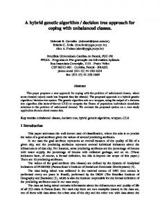
axis-parallel splits. Equally, a decision tree with more nodes is more difficult to comprehend than one with fewer nodes. Fig. 7 presents the average number of decision nodes for each of the data sets across the cost ratios (Table VII in the appendix provides standard errors). With

60 50 Tree Size

40 30 20 10

CSML

Fig. 7.

MC+AP

Io n M SP R EC I F W T D B W C PB C

Br ea st C

an ce r Bu pa Di CR ab X Ec ete ho s ca r G d Ha la s be s rm an He H ar e t-S ar ta t He tlo pa g t it i Ho s rs Ho e us e

0

MC+CSNL

ICET

Average tree size on data sets for each algorithm

the exception of two of the data sets, the results show that there is often a considerable improvement in the size of the tree induced by CSNL, which may help compensate for any loss of comprehensibility. However, this is only meant to be indicative and as Pazzani [2000] emphasises, it is unlikely that the “size of a model is the only factor that affects its comprehensibility”. Given that the non-linear decision nodes are more complex to compute than axis parallel splits, does their use not result in a much slower algorithm? Table II gives the average time taken by the algorithms for each data set. CSNL is significantly faster than the other algorithms, with an average of 1,643ms over all the data sets compared to an average above 10,000ms for the other algorithms, simply because it does not generate multiple trees. When MC+AP and MC+CSNL are compared, one might expect MC+CSNL to be much slower. However, as the results show, the fewer nodes required by MC+CSNL means that their time requirements are of a similar order and there is not much to choose between them.6 4. RELATED WORK AND BIBLIOGRAPHIC REMARKS Tree induction algorithms have a long history, with many papers and extensions, hence this section focuses only on the most related work. As mentioned in the introduction, much of the early research on decision tree learning focused on maximizing accuracy. Given the existence of this body of 6 Indeed,

each algorithm is better than the other for six of the data sets when a two-tailed student t-test at the 5% level is used.

14

·

Sunil Vadera

Table II. Average time of algorithms (milliseconds)± standard errors DATA SET CSNL MC+AP MC+CSNL ICET Breast Cancer 721 ± 37 8918 ± 48 7988 ± 313 9067 ± 379 Bupa 291 ± 20 2415 ± 61 3020 ± 121 3954 ± 46 CRX 6683 ± 266 17774 ± 107 29343 ± 1037 11849 ± 95 Diabetes 924 ± 65 17226 ± 112 9729 ± 880 19271 ± 59 EchoCard 158 ± 9 1963 ± 575 1066 ± 55 2018 ± 39 Glass 499 ± 22 2943 ± 28 2703 ± 174 3636 ± 29 Haberman 128 ± 8 1847 ± 17 1350 ± 94 2618 ± 94 Heart 1147 ± 96 8878 ± 90 8402 ± 643 5240 ± 15 Heart-StatLog 862 ± 47 7537 ± 41 7910 ± 545 2760 ± 17 Hepatitis 853 ± 53 5756 ± 548 7083 ± 304 3040 ± 42 Horse 1745 ± 154 19798 ± 85 17507 ± 1659 9076 ± 46 House 1432 ± 89 15252 ± 163 8553 ± 473 22427 ± 451 Ion 2282 ± 93 16493 ± 69 11197 ± 477 28613 ± 57 MRI 2300 ± 326 13178 ± 360 25020 ± 2271 13302 ± 307 SPECFT 4591 ± 638 24263 ± 324 43209 ± 6050 14898 ± 284 WDBC 930 ± 38 4458 ± 32 6949 ± 85 23467 ± 208 WPBC 2382 ± 232 18676 ± 238 12438 ± 884 15844 ± 321 work, a number of researchers have developed methods that aim to reduce a costsensitive problem to an equivalent accuracy maximization problem. One of the first proposals was by Breiman [1984], who suggested handling costs of misclassification by changing the distribution of the training examples to be equivalent to the ratio of costs of misclassification. More recently, Zadrozny et al. [2003] formalise this idea further, first by proving an elegant theorem which shows that minimizing the expected error rate of a revised distribution that reflects the relative costs is equivalent to minimizing the expected cost on the original distribution. They then take advantage of this theorem by developing a procedure, known as Costing, that utilizes rejection sampling to generate samples that reflect the relative costs. A base learner is then be applied to each sample and the classifiers produced are aggregated. Thus, as mentioned in Section 3, unlike MetaCost and CSNL, Costing does not output a single decision tree that can be interpreted as the decision making process. However, an advantage of the approach taken in Costing is that it can be applied to utilize not just existing accuracy based algorithms, but also any future algorithms. In this paper, the relationship between costs and proportion of examples is visible in equation(4), showing that stratifying the distribution can indeed have the same effect as including costs if CSNL is used. However, as the empirical trials in this paper and in Zadrozny et al. [2003] show, the nature of the base learner can make a significant difference to the extent which an overarching process (whether a GA, bagging, or stratification) succeeds in utilizing it to minimize costs. The algorithm developed in this paper caters only for costs of misclassification. The ICET system, which provides a comparison for our work, also takes account costs of carrying out tests and costs of delayed tests. Turney [2000] presents a

A Cost-Sensitive Non-Linear Decision Tree Algorithm

·

15

comprehensive taxonomy that includes other types of costs, such as costs that are conditional on time and costs of tests that are dependent on the outcome. Both noise and missing data can have a significant effect on learning algorithms. The study by Zhu et al. [2007] carries out an empirical evaluation of the effect of noise on cost-sensitive learning, concluding that costs of misclassification can magnify the effect of noise and therefore have a greater negative effect on minimizing costs. Ling et al. [2006] propose various strategies for obtaining missing values when the information can be obtained at a cost and carry out an empirical evaluation of their effectiveness when they are used with a cost-sensitive tree induction algorithm over discrete attributes. In addition to ICET and MetaCost, there are several other algorithms that consider costs of misclassification. As mentioned in the introduction, Pazzani et al. [1994] evaluate several extensions of accuracy based algorithms that take account of costs but conclude that they are no more effective than algorithms that ignore costs. They also develop an algorithm for ordering decision rules so as to minimize costs of misclassifications. Draper et al. [1994] present a cost-sensitive algorithm LMDT (Linear Machine Decision Trees) whose nodes consist of linear machines [Nilsson 1965]. A comparison of LMDT with ICET can be found in Vadera and Ventura [2001]. As well as MetaCost, several other systems utilize boosting to minimize costs of misclassification (e.g., [Ting and Zheng 1998; Fan et al. 1999; Ting 2000; Margineantu 2001; Merler et al. 2003]). For example, Fan et al. [1999] develop AdaCost, in which initial weights are allocated to examples to reflect the costs of misclassification. A learner, capable of taking account of weighted distributions of examples, is used to learn a classifier which is applied to the examples. The weights of examples that are correctly classified are reduced and weights of examples that are incorrectly classified and costly are increased. This process is then repeated, resulting in multiple classifiers which are used to provide a combined classification of the examples. Masnadi-Shirazi and Vasconcelos [2007] provide a theoretical analysis of these boosting algorithms. They argue that since the weight update equations utilised by these algorithms were developed heuristically, they do not necessarily converge to an optimal cost-sensitive decision boundary. Hence, instead, they propose a framework for the derivation of cost-sensitive boosting algorithms by first specifying a cost-sensitive loss function and then deriving cost-sensitive extensions of boosting algorithms by using gradient descent to minimise the loss function. The empirical evaluation shows that this leads to better results when compared with other boosting algorithms, such as AdaCost. Masnadi-Shirazi and Vasconcelos [2008] also develop an approach based on probability elicitation [Savage 1971], that allows the derivation of loss functions from the minimum conditional risk, and demonstrate it by developing a new boosting algorithm called SavageBoost that is shown to be less sensitive to outliers than AdaBoost. Section 3 uses a simple extension of reduced-error pruning that utilizes expected cost instead of error as the pruning criteria. The literature contains numerous methods for post-pruning which are surveyed in the paper by Breslow and Aha [1997b]. Empirical evaluations of the different pruning algorithms have been the subject of several studies, including those by Quinlan [1987], Mingers [1989], Esposito et al. [1997], and Breslow and Aha [1997a]. The reduced-error pruning

16

·

Sunil Vadera

method is regarded as a fast and simple method, though the technique used in C4.5 and ICET, known as error-based pruning, has been shown to perform particularly well [Breslow and Aha 1997a]. That is, no specific advantage was gained in using reduced-error pruning relative to ICET. A study by Frank and Witten [1998] shows that using data dependent significance tests in deciding whether to prune a subtree results in smaller trees without loss of accuracy, something that could be beneficial to algorithms that cater for costs of tests, though unlikely to aid minimization of costs of misclassification. The study also includes an excellent synthesis and discussion of the previous empirical research on pruning. The study by Pazzani et al. [1994] includes an evaluation of the effectiveness of cost-sensitive pruning on trees that utilize axis-parallel splits and concludes that it results in improvements for two of the four data sets used in their study. A later study, by Bradford et al. [1998], concludes that such pruning methods appear not to be effective in reducing costs, even relative to results from unpruned trees. A technical report [Vadera 2005a] presents results of the use of non-linear nodes, both before and after pruning and shows that cost-sensitive pruning does have a marked effect on reducing costs when non-linear nodes are utilized. There is growing interest in active learning, where a system needs to weigh the cost of acquiring new information against the cost of the final classification in a dynamic manner. Esmeir and Markovitch [2008] develop an algorithm for anytime induction of decision trees and carry out an empirical evaluation showing that it reduces classification cost with more time. Ji and Carin [2007] use partially observable Markov Decision Processes to formulate the cost-sensitive feature acquisition problem and develop a myopic algorithm that is computationally feasible. Kanani and Melville [2008] study a variation of the problem, where the task is to select the instances for which more information would lead to a reduction in classification cost at prediction time. Extension of CSNL so that it is able to perform active learning would require a more sophisticated approach to feature selection than it currently adopts and could be an interesting direction of future research. In Section 3, we compared ICET, MetaCost and CSNL by presenting their performance profiles as the ratios between the costs of misclassification vary from 0.0625 to 16.0. Though this is adequate for our purposes, several authors (e.g., [Provost et al. 1998; Martin et al. 1997]) have suggested the use of Receiver Operating Characteristic (ROC) curves [Swets 1964] so that the tradeoff between the false positives and the false negatives can be presented irrespective of costs, although Drummond and Holte [2006] point out some weaknesses of ROC curves and suggest an alternative visualisation called cost curves. 5. CONCLUSION The problem of developing a tree induction algorithm that takes account of costs of misclassifications has posed a significant challenge for the AI community, with over two decades of research and a number of variant approaches, mostly based on the use of axis-parallel splits. Experimental results, such as those by Pazzani et al. [1994], have shown that attempts to extend the information theoretic measure to include costs have not been effective and that to date, the best results have been obtained by using genetic algorithms to evolve trees, boosting or by bagging multiple trees.

A Cost-Sensitive Non-Linear Decision Tree Algorithm

·

17

This paper has presented a novel algorithm called CSNL that utilizes discriminant analysis to identify non-linear divisions that take account of costs of misclassifications. The algorithm is evaluated on 17 data sets and the results show that: —CSNL produces results comparable to ICET and MetaCost without evolving or generating multiple trees and in significantly less time. —Using bagging with CSNL produces results that improve upon those obtained by ICET and MetaCost on at least 12 of the 17 data sets. In general, the smaller trees induced by CSNL compensate for the cost of computing non-linear nodes, leading to similar time requirements to when MetaCost is used with an axisparallel base learner. The main current limitation of CSNL is that it only caters for two-class problems. Thus, methods of reducing multi-class problems to two classes, such as those investigated by Allwein et al. [2000] and Abe et al. [2004], need to be explored with CSNL. The algorithm focuses only on misclassification costs and future work could also consider other types of costs, such as costs of tests, and delayed costs [Turney 2000]. The discriminant used by CSNL is optimal if the multivariate normal condition is satisfied. It would therefore be interesting to develop a theory showing when CSNL is capable of producing good results, even when the data does not satisfy this condition. An independent empirical evaluation of the existing cost-sensitive algorithms that reveals their characteristics would also be a valuable addition to the literature. In conclusion, the new algorithm shows that the use of non-linear splits achieves a step improvement over the long established tradition of using axis-parallel divisions for inducing decision trees that take account of costs of misclassification. A. APPENDIX The appendix consists of the results for each data set in the form of average normalised costs, together with standard errors.

18

·

Sunil Vadera

Table III.

Results for the Breast Cancer Bupa CRX Diabetes and Echocard data

Ratio

ICET

MC+AP

0.06 0.13 0.25 0.50 1.00 2.00 4.00 8.00 16.00

8.43±0.63 8.48±0.74 9.23±0.69 11.16±0.62 14.69±0.86 12.01±0.65 9.80±0.50 9.65±0.70 7.96±0.67

2.58±0.32 3.97±0.44 6.83±0.49 9.72±0.74 13.99±0.91 11.74±0.70 7.99±0.48 6.47±0.55 4.34±0.43

0.06 0.13 0.25 0.50 1.00 2.00 4.00 8.00 16.00

21.20±1.79 21.35±2.08 21.55±1.28 25.43±1.39 32.55±1.80 25.98±1.35 20.86±1.32 17.98±1.49 15.94±1.56

10.06±1.54 13.40±1.22 18.39±1.30 24.69±1.65 37.88±3.07 23.08±1.77 16.40±1.35 12.62±1.37 6.66±1.20

0.06 0.13 0.25 0.50 1.00 2.00 4.00 8.00 16.00

17.49±1.03 18.13±0.99 20.94±1.22 24.50±1.10 32.11±1.16 24.48±0.81 19.38±0.71 17.84±0.93 16.97±0.75

7.49±0.47 11.39±0.62 16.36±0.76 23.25±0.90 33.65±1.44 23.57±0.90 16.90±0.58 11.60±0.59 7.55±0.42

0.06 0.13 0.25 0.50 1.00 2.00 4.00 8.00 16.00

49.17±1.48 50.90±1.44 52.80±1.17 62.73±1.39 74.58±1.40 48.48±1.17 35.87±1.63 27.38±2.28 29.27±3.18

16.44±0.98 28.04±1.03 41.09±1.24 57.91±0.91 79.84±1.28 48.43±1.20 28.12±0.72 18.85±1.05 9.89±0.55

0.06 0.13 0.25 0.50 1.00 2.00 4.00 8.00 16.00

31.22±6.02 38.41±6.09 47.59±5.22 71.05±4.45 112.23±5.17 88.31±5.22 82.35±5.43 74.25±5.25 75.44±5.63

11.86±2.08 19.94±2.45 41.57±3.96 69.14±4.04 124.28±8.35 90.69±5.59 64.94±4.03 48.57±4.13 34.46±3.71

CSNL MC+CSNL Breast Cancer 3.22±0.35 3.75±0.09 4.75±0.49 5.94±0.35 6.66±0.54 6.28±0.48 8.88±0.56 8.34±0.55 14.72±1.00 14.16±1.00 9.24±0.61 9.97±0.71 8.67±0.61 8.19±0.45 5.96±0.41 5.67±0.30 4.78±0.46 4.43±0.20 Bupa 11.79±1.34 6.15±0.15 19.13±1.35 12.85±0.61 24.90±1.22 23.55±1.53 33.90±1.38 31.03±1.92 41.26±2.49 42.78±3.00 29.84±1.72 28.91±1.44 18.13±1.22 17.25±0.84 11.27±1.18 10.34±0.72 7.00±0.95 7.21±0.32 CRX 8.47±0.53 8.15±0.19 11.69±0.50 12.78±0.41 14.86±0.63 14.09±0.63 21.47±0.73 20.53±0.72 35.52±0.99 33.00±1.09 24.91±1.19 23.94±0.83 18.33±0.83 19.23±0.59 10.89±0.50 10.96±0.28 7.13±0.41 6.29±0.11 Diabetes 11.48±0.12 11.68±0.11 20.37±0.47 23.25±0.18 32.90±0.59 41.42±0.64 54.38±1.12 55.82±0.98 72.52±1.02 74.56±1.30 43.87±0.72 44.47±0.64 25.21±0.49 25.38±0.35 14.55±0.37 12.80±0.23 7.21±0.28 6.30±0.08 EchoCard 12.84±2.68 6.19±0.37 16.51±1.80 12.39±0.73 36.11±3.33 28.55±3.29 61.30±4.98 52.06±2.99 113.65±6.69 104.69±6.53 91.53±4.62 93.77±4.46 75.16±5.20 70.12±3.99 52.41±4.12 54.30±1.64 42.20±3.06 27.78±0.38

CSNL3

MC+CSNL3

3.30±0.29 4.56±0.32 5.84±0.39 8.23±0.51 12.53±1.03 9.89±0.63 9.03±0.60 6.46±0.65 5.69±0.66

3.03±0.18 3.98±0.25 5.67±0.39 7.89±0.52 11.69±0.82 10.48±0.77 7.81±0.61 5.56±0.30 4.35±0.15

11.30±1.49 21.01±1.52 25.45±1.45 31.03±1.81 43.62±2.19 27.73±1.95 16.65±1.13 13.44±1.29 8.70±1.51

6.14±0.15 12.96±0.76 19.49±1.26 28.41±1.65 41.09±1.99 25.28±1.51 17.88±1.13 11.60±0.78 8.03±0.50

8.52 ± 0.63 11.66 ± 0.58 14.85 ± 0.49 24.16 ±0.96 37.08±1.11 26.26±1.05 17.18± 0.54 11.71 ±0.54 8.08 ± 0.51

8.17±0.28 12.83±0.43 14.96±0.62 21.34±0.64 33.96±1.21 22.16±0.77 18.31±0.53 10.83±0.27 6.43±0.15

10.42 ± 0.17 18.43 ± 0.54 32.49 ± 0.69 52.86 ± 1.17 72.47±1.35 44.86±1.03 25.40±0.43 14.33±0.3 7.14±0.25

11.56±0.09 21.35±0.23 35.19±0.54 54.28±1.04 72.97±1.41 45.47±0.56 26.02±0.43 12.87±0.22 6.30±0.08

13.40±3.66 20.43±2.44 38.07±4.04 61.58±4.21 105.25±6.72 88.73±6.10 81.18±4.99 53.74±4.58 36.67±3.18

6.19±0.37 12.39±0.73 26.31±1.46 51.5±2.99 110.85±6.62 94.89±5.59 71.24±3.74 52.13±2.68 27.78±0.45

A Cost-Sensitive Non-Linear Decision Tree Algorithm Table IV.

·

19

Results for the Glass Haberman Heart Heart-StatLog and Hepatitis data

Ratio

ICET

MC+AP

0.06 0.13 0.25 0.50 1.00 2.00 4.00 8.00 16.00

31.56±2.67 30.17±1.97 33.40±2.58 38.88±2.13 47.84±2.48 37.29±2.15 31.60±2.26 25.88±1.79 24.55±2.04

11.94±1.44 19.12±2.02 26.51±2.14 39.60±2.71 55.08±3.13 36.00±2.04 24.12±1.46 20.07±2.44 11.06±1.23

0.06 0.13 0.25 0.50 1.00 2.00 4.00 8.00 16.00

72.30±3.10 71.74±3.16 79.39±2.93 87.46±2.84 105.97±3.08 52.19±2.44 25.56±1.37 11.84±0.33 6.75±0.83

30.24±1.89 49.01±2.31 67.24±2.84 88.88±2.47 110.23±3.23 63.64±2.12 30.91±1.22 17.73±1.23 9.22±0.67

0.06 0.13 0.25 0.50 1.00 2.00 4.00 8.00 16.00

26.30±1.56 29.54±1.54 31.68±1.19 40.09±1.50 51.11±2.27 35.46±1.60 31.29±1.52 25.26±1.58 26.21±1.98

10.79±0.81 18.33±1.33 29.39±1.77 37.95±1.54 54.00±1.94 37.90±2.25 20.42±0.94 14.24±0.97 9.08±0.79

0.06 0.13 0.25 0.50 1.00 2.00 4.00 8.00 16.00

27.54±1.66 28.82±1.57 33.44±1.69 38.44±1.57 47.96±1.34 36.25±1.85 28.93±1.16 29.72±1.60 24.22±1.30

12.57±1.12 21.32±1.48 31.58±1.84 41.11±1.79 54.56±2.41 34.83±1.47 23.03±1.20 15.53±0.94 8.55±0.67

0.06 0.13 0.25 0.50 1.00 2.00 4.00 8.00 16.00

42.64±3.02 41.54±2.78 44.65±3.37 56.12±3.25 65.68±3.21 46.99±3.40 31.65±2.85 30.08±3.45 18.32±2.69

43.86±3.91 40.70±4.37 52.83±3.75 67.17±4.46 89.14±4.88 58.59±4.39 32.22±3.09 19.04±1.95 13.16±1.94

CSNL MC+CSNL Glass 11.01±1.33 7.01±0.17 18.04±1.55 13.95±0.35 25.79±1.90 27.14±0.75 36.72±2.51 38.34±2.59 53.28±2.50 47.70±2.43 35.01±1.58 43.56±1.54 24.26±1.16 24.17±0.85 15.12±1.16 12.35±0.35 13.49±1.54 6.48±0.17 Haberman 19.05±0.72 17.49±0.17 38.27±1.21 35.09±0.31 68.23±2.30 68.32±1.35 81.76±3.13 80.27±2.35 98.32±2.40 96.83±2.41 57.02±1.54 52.05±1.64 30.99±1.57 25.82±1.13 18.58±1.31 12.23±0.35 13.59±1.72 6.69±0.64 Heart 11.21±0.97 7.37±0.11 17.51±1.18 14.54±0.30 24.92±1.21 24.21±0.84 35.90±1.42 35.95±1.26 52.43±2.10 51.94±1.72 36.39±1.57 35.31±1.53 22.65±1.27 21.84±0.63 14.72±1.15 12.06±0.45 9.95±0.74 6.15±0.13 Heart-StatLog 10.84±0.77 7.85±0.13 18.72±0.93 15.99±0.50 27.22±1.21 26.11±1.09 36.00±1.63 39.44±1.25 55.56±2.37 52.22±2.02 35.50±1.45 35.56±1.20 24.39±1.21 23.33±0.56 13.82±0.69 12.78±0.49 10.02±1.01 6.17±0.12 Hepatitis 29.79±2.78 23.36±0.85 41.64±3.74 36.20±2.04 55.13±2.77 44.99±2.29 65.91±4.44 62.98±3.82 87.04±5.25 80.35±5.01 49.80±3.50 45.61±2.34 33.06±3.10 25.00±1.57 18.20±2.12 12.08±0.63 14.12±2.24 6.07±0.32

CSNL3

MC+CSNL3

9.14±1.05 19.44±1.85 25.16±1.19 38.25±2.08 51.30±3.02 37.89±1.70 25.74±1.27 15.14±1.04 7.59±0.68

7.01±0.17 13.34±0.44 26.46±1.55 32.67±1.84 49.14±2.33 40.41±2.15 23.27±0.93 12.38±0.41 6.42±0.19

19.98±1.21 37.16±1.29 65.38±2.17 81.27±3.08 96.16±3.17 57.10±1.94 31.78±1.60 18.31±1.17 11.48±1.16

17.49±0.17 35.44±0.38 65.09±1.31 78.95±2.29 97.16±2.75 52.55±1.65 24.16±0.67 13.05±0.74 6.04±0.17

10.50±0.89 16.80±1.07 25.53±1.37 35.70±1.43 49.59±2.17 33.60±1.60 22.50±1.28 15.97±1.14 10.33±0.82

7.65±0.31 14.95±0.76 22.82±1.44 33.94±1.28 48.13±2.27 31.64±1.32 19.25±0.73 12.12±0.59 6.15±0.23

11.19±0.99 18.90±1.05 25.81±1.38 36.33±1.51 51.78±1.83 35.33±0.99 24.69±1.26 14.83±1.06 10.96±0.86

8.51±0.58 15.72±0.81 25.53±1.17 36.11±1.44 49.11±1.75 32.44±1.48 21.92±0.88 12.56±0.73 6.44±0.34

31.91±3.12 35.15±2.81 47.6±3.04 66.54±4.46 79.09±5.20 50.01±3.68 35.99±3.36 23.49±3.27 14.59±2.15

26.76±2.23 36.62±2.55 47.5±4.09 61.10±4.73 81.60±4.23 49.17±2.85 29.19±1.8 13.91±1.03 6.07±0.32

20

·

Sunil Vadera

Table V.

Results for Horse House Ion MRI data

Ratio

ICET

MC+AP

0.06 0.13 0.25 0.50 1.00 2.00 4.00 8.00 16.00

32.68±1.89 38.19±1.72 36.96±1.35 43.40±1.27 58.32±2.68 42.66±1.16 37.00±1.51 29.17±1.46 27.13±2.04

13.17±0.81 22.01±0.83 35.70±1.96 48.62±1.90 69.87±2.76 46.85±1.68 30.60±1.21 19.41±1.08 10.27±0.66

0.06 0.13 0.25 0.50 1.00 2.00 4.00 8.00 16.00

24.37±2.13 26.10±2.09 31.67±2.14 39.26±1.49 44.75±1.41 30.79±1.21 22.72±1.15 18.39±1.26 15.16±1.18

7.05±0.58 12.57±0.94 18.92±1.04 28.44±1.54 35.95±1.34 22.68±0.99 12.13±0.47 8.67±0.58 4.17±0.20

0.06 0.13 0.25 0.50 1.00 2.00 4.00 8.00 16.00

18.56±1.02 18.50±0.65 18.92±0.95 20.72±1.16 26.53±1.59 19.10±0.85 15.02±1.18 13.89±1.04 13.43±1.24

22.47±6.54 29.26±5.63 33.55±5.48 39.84±4.23 54.90±6.68 47.47±7.05 31.66±6.01 30.30±6.14 20.63±5.38

0.06 0.13 0.25 0.50 1.00 2.00 4.00 8.00 16.00

64.86±2.00 63.83±2.33 69.91±2.40 81.08±3.10 100.39±3.52 55.71±2.07 40.99±3.22 29.11±2.46 22.02±3.14

28.62±1.73 55.18±2.30 70.88±2.57 87.11±2.71 100.37±2.73 61.17±2.66 29.16±1.22 18.30±1.31 8.71±0.86

CSNL MC+CSNL Horse 11.07±0.49 9.94±0.13 20.84±0.78 19.86±0.27 34.94±1.12 35.37±1.01 50.09±1.35 49.24±1.28 68.82±2.46 69.02±1.86 47.57±1.71 47.04±1.07 30.17±1.28 25.79±0.56 17.13±0.94 13.05±0.35 8.46±0.58 6.44±0.13 House 6.55±0.34 5.47±0.15 9.29±0.35 9.58±0.28 14.85±0.62 15.25±0.41 24.31±1.06 23.66±0.81 35.95±1.69 35.56±1.39 21.51±0.81 22.65±0.77 13.87±0.56 18.92±0.62 9.77±0.38 12.52±0.28 5.40±0.18 6.79±0.12 Ion 15.46±4.19 8.56±0.64 24.55±6.16 16.60±1.05 31.12±4.54 30.82±5.22 46.18±7.10 44.99±5.77 55.70±8.11 60.65±8.39 40.53±6.52 42.32±6.98 31.27±6.16 31.91±5.79 26.39±6.73 15.29±2.39 19.71±5.89 6.11±0.50 MRI 22.84±1.09 21.21±0.17 37.82±1.25 41.01±0.61 68.79±2.10 63.88±1.41 92.38±2.69 89.67±2.73 101.54±2.34 103.15±2.53 55.82±2.15 51.06±1.32 29.01±1.08 25.02±0.67 17.77±1.38 12.66±0.35 11.48±1.26 6.25±0.17

ACM Journal Name, Vol. V, No. N, August 2009.

CSNL3

MC+CSNL3

11.12±0.59 21.08±1.01 34.63±1.16 52.29±1.51 76.07±3.16 50.86±1.63 29.88±1.45 17.64±0.9 8.43±0.80

9.93±0.13 19.27±0.38 30.60±0.89 50.14±1.88 69.11±2.56 47.00±1.27 26.52±0.69 13.00±0.25 6.44±0.13

6.88±0.44 10.41±0.64 16.41±0.87 25.31±1.18 35.62±1.58 21.29±0.64 15.28±0.73 9.31±0.63 5.92±0.41

5.75±0.17 9.18±0.34 14.79±0.43 24.53±0.92 35.13±1.25 22.46±0.75 16.67±0.47 11.03±0.29 6.88±0.13

17.55±5.07 16.4±1.69 22.94±2.44 36.17±4.33 61.05±8.79 43.01±7.59 30.13±6.33 28.62±7.26 18.71±6.24

8.35±0.51 15.41±0.95 24.88±1.91 37.46±4.14 65.41±8.21 46.78±7.12 28.74±5.34 15.76±2.84 6.08±0.51

24.40±1.11 42.67±1.46 68.42±2.64 94.65±2.88 102.42±3.15 56.04±2.08 31.98±1.92 18.17±1.76 11.30±1.35

21.43±0.35 39.19±0.84 63.96±1.56 90.70±2.59 101.39±2.86 53.11±1.83 25.02±0.67 12.51±0.34 6.25±0.17

A Cost-Sensitive Non-Linear Decision Tree Algorithm

Table VI.

·

21

Result for SPECFT WDBC WPBC data

Ratio

ICET

MC+AP

0.06 0.13 0.25 0.50 1.00 2.00 4.00 8.00 16.00

28.17±2.79 32.43±3.52 39.23±2.74 56.58±1.84 82.28±3.17 60.08±1.66 54.34±2.24 51.53±2.59 45.17±1.97

171.02±36.26 60.42±23.49 35.75±2.79 65.42±4.00 112.80±4.76 89.41±3.95 62.98±2.38 49.00±2.49 24.96±2.13

0.06 0.13 0.25 0.50 1.00 2.00 4.00 8.00 16.00

9.62±0.51 10.43±0.61 10.44±0.55 11.70±0.58 15.02±0.94 11.26±0.61 10.84±0.79 8.40±0.73 8.48±0.69

5.58±0.81 10.84±1.56 17.55±2.18 19.07±1.95 27.47±2.78 19.45±1.75 10.81±1.15 8.90±1.70 3.88±0.74

0.06 0.13 0.25 0.50 1.00 2.00 4.00 8.00 16.00

64.61±3.49 65.29±3.15 71.72±4.08 85.57±2.56 96.08±3.83 57.31±2.91 31.91±2.54 20.18±2.28 15.37±3.22

24.82±2.24 57.93±5.49 73.77±5.43 100.08±6.37 112.70±5.09 62.95±3.99 34.41±1.53 19.36±1.65 9.36±1.01

CSNL SPECFT 6.30±0.27 12.61±0.54 25.76±1.17 63.47±2.28 113.29±4.08 81.74±3.96 57.99±2.29 39.83±2.93 23.45±2.29 WDBC 7.63±1.23 8.49±1.16 13.03±1.52 17.67±1.36 27.47±2.73 17.29±1.49 13.67±1.99 11.48±1.91 7.30±1.55 WPBC 17.82±1.80 35.88±3.58 69.40±4.67 100.23±5.56 117.00±6.41 67.96±3.53 37.35±2.43 18.28±1.39 8.28±0.53

MC+CSNL

CSNL3

MC+CSNL3

6.30±0.27 12.61±0.54 25.22±1.09 52.87±2.34 103.30±4.03 78.09±3.62 59.63±2.30 33.01±0.86 19.58±0.51

6.30±0.27 14.37±1.06 36.06±2.20 67.00±2.61 114.27±4.89 80.64±4.03 61.58±2.79 38.25±2.85 25.05±1.82

6.30±0.27 12.61±0.54 25.95±1.28 53.84±2.14 101.84±5.45 78.82±3.08 51.83±1.88 30.52±1.03 17.91±0.61

9.25±0.81 10.59±0.91 13.29±1.29 20.98±2.10 26.96±2.47 18.06±1.73 8.52±1.21 8.81±1.42 3.54±0.30

4.07±0.47 5.59±0.40 8.45±0.50 12.92±0.65 17.21±0.72 12.20±0.81 8.38±0.64 5.53±0.45 5.21±0.54

6.42±0.28 6.78±0.20 7.85±0.34 12.99±0.75 18.34±0.87 11.66±0.59 8.89±0.45 5.39±0.29 4.02±0.32

12.87±0.29 26.92±0.75 45.96±2.42 93.63±4.44 117.58±5.76 63.09±2.46 30.97±1.17 15.49±0.58 7.74±0.29

22.67±2.80 35.42±2.81 73.27±3.11 91.19±4.50 111.27±4.75 61.08±3.65 35.49±1.97 16.88±1.12 9.36±1.20

12.87±0.29 25.67±0.59 55.06±2.57 83.16±5.12 116.14±5.56 62.95±2.53 30.97±1.17 15.49±0.58 7.74±0.29

·

22

Sunil Vadera Table VII.

DATA BreastCan Bupa CRX Diabetes EchoCard Glass Haberman Heart Heart-Stat Hepatitis Horse House Ion MRI SPECFT WDBC WPBC

Table VIII. Ratio 0.06 0.13 0.25 0.50 1.00 2.00 4.00 8.00 16.0

Average number of nodes ± standard errors on data sets

CSNL 11.7 ± 1.1 9.8 ± 1.1 16.8 ± 2.0 10.1 ± 2.2 6.6 ± 0.7 12.9 ± 1.3 9.4 ± 1.2 12.4 ± 1.4 11.1 ± 1.4 7.8 ± 0.8 12.6 ± 2.7 12.5 ± 2.0 7.8 ± 0.5 11.2 ± 1.9 6.2 ± 1.5 6.1 ± 0.3 6.8 ± 0.9

MC+AP 18.5 ± 0.7 11.9 ± 0.5 31.0 ± 1.2 45.4 ± 4.7 10.6 ± 1.3 15.7 ± 0.5 31.5 ± 5.3 22.7 ± 1.1 20.9 ± 0.8 10.2 ± 1.0 27.2 ± 1.8 25.1 ± 1.2 8.8 ± 0.2 20.8 ± 3.3 12.3 ± 1.4 6.1 ± 0.3 9.4 ± 1.5

MC+CSNL 11.3 ± 0.5 11.9 ± 0.5 13.2 ± 1.9 7.0 ± 1.8 4.1 ± 1.0 4.3 ± 1.1 4.5 ± 1.3 8.9 ± 1.8 8.3 ± 1.6 5.5 ± 1.0 7.6 ± 2.2 8.3 ± 1.5 5.9 ± 0.8 6.5 ± 2.5 5.2 ± 1.3 5.3 ± 0.2 4.3 ± 1.4

ICET 20.3 ± 1.3 16.5 ± 0.3 27.5 ± 2.5 55.6 ± 14.1 10.3 ± 1.6 21.7 ± 0.7 17.9 ± 5.1 30.7 ± 1.5 25.5 ± 1.4 13.2 ± 1.2 44.0 ± 2.7 6.0 ± 0.6 22.8 ± 0.4 31.2 ± 7.1 23.6 ± 2.7 18.1 ± 0.4 17.7 ± 4.7

CSNL3 10.7 ± 0.8 9.5 ± 0.6 19.3 ± 2.3 10.6 ± 2.5 6.7 ± 0.6 8.5 ± 1.2 10.4 ± 1.4 11.7 ± 1.2 11.4 ± 1.2 7.9 ± 0.4 13.1 ± 2.3 11.2 ± 1.5 6.8 ± 0.3 9.8 ± 1.7 6.8 ± 1.2 9.0 ± 0.5 6.0 ± 0.7

MC+CSNL3 9.8± 0.4 6.5 ± 0.8 14.0 ± 1.0 7.9 ± 1.7 3.6 ± 0.8 5.3 ± 1.0 5.0 ± 1.4 11.3 ± 1.3 10.3 ± 1.2 5.5 ± 0.8 9.2 ± 2.05 8.7 ± 1.1 4.8 ± 0.5 6.5 ± 2.0 5.8 ± 1.3 7.5 ± 0.5 3.2± 0.9

Comparison of Accuracies for the ION data set for ICET, CSNL, MC+AP ICET %Acc %Acc C1 C2

%Acc 88.8 89.3 89.2 90.1 89.3 89.0 88.6 88.3 87.7

93.4 93.6 92.7 94.6 93.3 93.8 93.9 93.0 92.6

79.9 80.6 81.9 81.0 81.4 79.6 78.5 78.8 78.2

Cost

%Acc

18.6 18.5 18.9 20.7 26.5 19.1 15.0 13.9 13.4

55.4 62.5 68.4 71.1 75.6 75.6 73.0 73.7 69.9

CSNL %Acc %Acc C1 C2 28.1 47.1 55.5 70.2 72.9 80.1 82.5 82.6 87.7

91.6 85.2 82.0 75.5 76.9 69.0 61.1 60.2 50.2

Cost

%Acc

15.5 24.6 31.1 46.2 55.7 40.5 31.3 26.4 19.7

58.4 66.7 68.0 72.3 75.9 72.2 69.7 67.3 64.8

MC+AP %Acc %Acc C1 C2 39.9 58.4 60.7 63.2 75.3 75.8 85.8 80.8 87.3

Table IX. Pairwise comparison of CSNL3 with other algorithms using a two-tailed student t-test at p = 0.05 level WPBC

WDBC

SPEC

MRI

ION

HOUSE

HORSE

HEPA

H’T-ST

HEART

HABER

GLASS

ECHO

DIAB

CRX

BUPA

BC

ALGORITHM MC+AP better

0

3

0

0

1

0

0

0

1

0

0

2

0

0

0

0

0

CSNL3 better

0

0

0

9

0

1

4

0

1

1

0

0

1

1

2

5

1

MC+AP better

0

0

0

0

0

0

0

0

0

0

0

3

0

0

0

0

0

MC+CSNL3 better

0

1

1

9

4

5

8

5

6

3

6

4

4

7

7

5

5

ICET better

0

2

1

0

0

0

3

0

0

1

3

0

4

1

3

0

1

CSNL3 better

7

4

6

8

4

3

4

7

6

1

5

9

0

5

4

6

2

ICET better

0

1

0

0

0

0

0

0

0

1

3

0

5

1

2

1

1

MC+CSNL better

8

4

7

8

6

7

5

7

6

3

6

9

3

6

5

6

4

CSNL better

0

0

1

0

0

0

0

0

0

0

0

0

0

1

1

0

0

CSNL3 better

0

0

0

2

0

1

0

0

0

0

0

0

0

0

0

8

0

83.5 77.1 80.8 82.5 72.1 68.7 50.7 48.2 35.5

Cost 22.5 29.3 33.6 39.8 54.9 47.5 31.7 30.3 20.6

A Cost-Sensitive Non-Linear Decision Tree Algorithm

·

23

REFERENCES Abe, N., Zadrozny, B., and Langford, J. 2004. An iterative method for multi-class costsensitive learning. In Proc. of KDD, Seattle, Washington. 3–11. Allwein, E. L., Schapire, R. E., and Singer, Y. 2000. Reducing multiclass to binary: A unifying approach for margin classifiers. In Proc. 17th Int. Conf. on Machine Learning. San Francisco: Morgan Kaufmann, 9–16. Althoff, K., Auriol, E., Barletta, R., and Manago, M. 1995. A review of industrial casebased reasoning tools. Oxford: AI Intelligence. Bauer, E. and Kohavi, R. 1999. An empirical comparison of voting classification algorithms: Bagging, boosting, and variants. Machine Learning 36, 1-2, 105–139. Bennett, K. P. 1999. On mathmatical programming methods and support vector machines. In Advances in Kernel Methods – Support Vector Machines, A. Schoelkopf, C. Burges, and A. Smola, Eds. Cambridge, MA:MIT Press, Chapter 19, 307–326. Berry, M. and Linoff, G. 2004. Data Mining Techniques, 2nd ed. New York : Wiley. Blake, C. and Merz, C. 1998. UCI Repository of Machine Learning Databases. Irvine, CA: University of California, Department of Information and Computer Science, USA, available at //www.ics.uci.edu/ mlearn/ MLRepository.html. Bradford, J., Kunz, C., Kohavi, R., Brunk, C., and Brodley, C. 1998. Pruning decision trees with misclassification costs. In Proc. of the 10th European Conf. on Machine Learning, Chemnitz, Germany, Lecture Notes in Computer Science, No 1398. Heidelberg:Springer Verlag, 131–136. Breiman, L. 1996. Bagging predictors. Machine Learning 24, 2, 123–140. Breiman, L., Friedman, J. H., Olsen, R. A., and Stone, C. J. 1984. Classification and Regression Trees. Belmont: Wadsworth. Breslow, L. and Aha, D. 1997a. Comparing tree-simplification procedures. In Proc. of the 6th Int. Workshop on Artificial Intelligence and Statistics, Ft. Lauderdale, Florida. 67–74. Breslow, L. and Aha, D. 1997b. Simplifying decision trees: A survey. Knowledge Engineering Review 12, 1–40. Brown, G. 2009. Feature selection by filters: a unifying perspective. In Proc. of the 5th UK Symposium on Knowledge Discovery and Data Mining, S. Vadera, Ed. University of Salford, UK, 34–43. Dash, M. and Liu, H. 1997. Feature selection for classification. Intelligent Data Analysis 1, 3, 131–156. Domingos, P. 1999. MetaCost: A general method for making classifiers cost-sensitive. In Proc. of the 5th Int. Conf. on Knowledge Discovery and Data Mining. 155–164. Draper, B., Brodley, C. E., and Utgoff, P. E. 1994. Goal-directed classification using linear machine decision trees. IEEE Transactions on Pattern Analysis and Machine Intelligence 16, 9, 888–893. Drummond, C. and Holte, R. 2006. Cost curves: An improved method for visualizing classifier performance. Machine Learning 65, 1, 95–130. Elkan, C. 2001. The foundations of cost-sensitive learning. In Proc. of the 17th Int. Joint Conf. on Artificial Intelligence. San Francisco : Morgan Kaufmann, 973–978. Esmeir, S. and Markovitch, S. 2008. Anytime induction of low-cost, low-error classifiers: a sampling-based approach. Journal of Artificial Intelligence Research (JAIR) 33, 1–31. Esposito, F., Malerba, D., and Semeraro, G. 1997. A compartive analysis of methods for pruning decision trees. IEEE Transactions on Pattern Analysis and Machine Intelligence 19, 5, 476–491. Fan, W., Stolfo, S., Zhang, J., and Chan, P. 1999. AdaCost: Misclassification cost-sensitive boosting. In Proc. of the 16th Int. Conf. on Machine Learning. San Francisco : Morgan Kaufmann, 97–105. Fisher, R. 1936. The use of multiple measurements in taxonomic problems. Annals of Eugenics 8, 179–188.

24

·

Sunil Vadera

Frank, E. and Witten, I. 1998. Reduced-error pruning with significance tests, available at http://citeseer.ist.psu.edu/frank98reducederror.html. Grefenstette, J. 1986. Optimization of control parameters for genetic algorithms. IEEE Transactions on Systems, Man, and Cybernetics 16, 122–128. Hong, S. J. 1997. Use of contextual information for feature ranking and discretization. IEEE Transactions on Knowledge and Data Engineering 9, 718–730. Ji, S. and Carin, L. 2007. Cost-sensitive feature acquisition and classification. Pattern Recognition 40, 5, 1474–1485. Johnson, R. and Wichern, D. 1998. Applied Multivariate Statistical Analysis, 4th ed. Englewood Cliffs:Prentice Hall. Kanani, P. and Melville, P. 2008. Prediction-time active feature-value acquisition for customer targeting. In Proc. of the Workshop on Cost Sensitive Learning, NIPS 2008, available at http://www.cs.iastate.edu/ oksayakh/csl/accepted papers/kanani.pdf. Knoll, U., Nakhaeizadeh, G., and Tausend, B. 1994. Cost-sensitive pruning of decision trees. In Proc. of the 8th European Conf. on Machine Learning. Vol. 2. Berlin:Springer-Verlag, 383– 386. Kohavi, R. and John, G. H. 1997. Wrappers for feature subset selection. Artificial Intelligence 97, 1-2, 273–324. Ling, C., Sheng, V., and Yang, G. 2006. Test strategies for cost-sensitive decision trees. IEEE Transactions on Knowledge and Data Engineering 18, 8, 1055–1067. Margineantu, D. 2001. Methods for cost-sensitive learning. Ph.D. thesis, School of Electrical Engineering and Computer Science, Oregan State University, Corvallis, USA. Martin, A., Doddington, G., Kamm, T., Ordowski, M., and Przybocki, M. 1997. The DET curve in assessment of detection task performance. In Proc. of Eurospeech ’97. Int. Speech Communications Association, Bonn, Germany, Rhodes, Greece, 1895–1898. Masnadi-Shirazi, H. and Vasconcelos, N. 2007. Asymmetric boosting. In Proc. of 24th Int. Conf. on Machine Learning. 609–616. Masnadi-Shirazi, H. and Vasconcelos, N. 2008. On the design of loss functions for classification: theory, robustness to outliers, and SavageBoost. In Proc. of Neural Information Processing Systems, D. Koller, D. Schuurmans, Y. Bengio, and L. Bottou, Eds. 1049–1056. Merler, S., Furlanello, C., Larcher, B., and Sboner, A. 2003. Automatic model selection in cost-sensitive boosting. Information Fusion 4, 3–10. Mingers, J. 1989. An empirical comparison of pruning methods for decision tree induction. Machine Learning 4, 227–243. Murthy, S., Kasif, S., and Salzberg, S. 1994. A system for induction of oblique decision trees. Journal of Artificial Intelligence Research 2, 1–32. Nilsson, N. 1965. Learning Machines. New York : McGraw-Hill. ´n ˜ ez, M. 1991. The use of background knowledge in decision tree induction. Machine LearnNu ing 6, 231–250. Pazzani, M., Merz, C., Murphy, P., Ali, K., Hurne, T., and Brunk, C. 1994. Reducing misclassification costs: Knowledge-intensive approaches to learning from noisy data. In Proc. of the 11th Int. Conf. on Machine Learning. San Francisco: Morgan Kaufmann, 217–225. Pazzani, M. J. 2000. Knowledge discovery from data? IEEE Intelligent Systems 15, 2, 10–13. Provost, F. J. and Buchanan, B. G. 1995. Inductive policy: The pragmatics of bias selection. Machine Learning 20, 35–61. Provost, F. J., Fawcett, T., and Kohavi, R. 1998. The case against accuracy estimation for comparing induction algorithms. In Proc. of the 15th Int. Conf. on Machine Learning. 445–553. Quinlan, J. R. 1987. Simplifying decision trees. Int. Journal of Man-Machine Studies 27, 221–234. Quinlan, J. R. 1993. C4.5 : Programs for Machine Learning. California:Morgan Kauffman. Savage, L. 1971. The elicitation of personal probabilities and expectations. Journal of the American Statistical Association 66, 783–801. Swets, J. 1964. Signal Detection and Recognition by Human Observers. John Wiley & Sons Inc.

A Cost-Sensitive Non-Linear Decision Tree Algorithm

·

25

Tan, M. 1993. Cost-sensitive learning of classification knowledge and its applications in robotics. Machine Learning 13, 7–33. Ting, K. 2000. A comparative study of cost-sensitive boosting algorithms. In Proc. of the 17th Int. Conf. on Machine Learning. San Francisco : Morgan Kaufmann, 983–990. Ting, K. and Zheng, Z. 1998. Boosting trees for cost-sensitive classifications. In Proc. of the 10th European Conf. on Machine Learning. 190–195. Turney, P. 1995. Cost sensitive classification: Empirical evaluation of a hybrid genetic decision tree induction algorithm. Journal of Artificial Intelligence Research 2, 369–409. Turney, P. 2000. Types of cost in inductive concept learning. In Proc. of the Workshop on Cost-Sensitive Learning, 7th Int. Conf. on Machine Learning. 15–21. Vadera, S. 2005a. Inducing Cost-Sensitive Nonlinear Decision Trees, Technical Report. School of Computing, Science and Engineering, University of Salford. Vadera, S. 2005b. Inducing safer oblique trees without costs. The International Journal of Knowledge Engineering and Neural Networks 22, 4, 206–221. Vadera, S. and Ventura, D. 2001. A comparison of cost-sensitive decision tree learning algorithms. In Proc. of the 2nd European Conf. on Intelligent Management Systems in Operations. Operational Research Society, Birmingham, UK, 79–86. W.Buntine and Niblett, T. 1992. A further comparison of splitting rules for decision-tree induction. Machine Learning 8, 75–85. Zadrozny, B., Langford, J., and Abe, N. 2003. Cost-sensitive learning by cost-proportionate example weighting. In Proc. of the 3rd IEEE International Conference on Data Mining. 435– 442. Zhu, X., Wu, X., Khoshgoftaar, T., and Shi, Y. 2007. An empirical study of noise impact on cost-sensitive learning. In Proc. of 20th Int.Joint Conf. on Artificial Intelligence. 1168–1174. ACKNOWLEDGMENT

The author is most grateful to his MSc students, David Ventura who re-implemented ICET, and to Matt Gallagher who helped implement an earlier of version the algorithm. The author is also grateful to the reviewers and associate editors whose comments have led to significant improvements to the paper.