CT-ITL: Efficient Frequent Item Set Mining Using a ... - CiteSeerX

CT-ITL: Efficient Frequent Item Set Mining Using a Compressed Prefix Tree with Pattern Growth Yudho Giri Sucahyo Raj P. Gopalan School of Computing Curtin University of Technology Bentley, Western Australia 6102 {sucahyoy, raj}@curtin.computing.edu.au

Abstract Discovering association rules that identify relationships among sets of items is an important problem in data mining. Finding frequent item sets is computationally the most expensive step in association rule discovery and therefore it has attracted significant research attention. In this paper, we present a more efficient algorithm for mining complete sets of frequent item sets. In designing our algorithm, we have modified and synthesized a number of useful ideas that include prefix trees, patterngrowth, and tid-intersection. We extend the prefix-tree structure to store transaction groups and propose a new method to compress the tree. Transaction-id intersection is modified to include the count of transaction groups. We present performance comparisons of our algorithm against the fastest Apriori algorithm, Eclat and the latest extension of FP-Growth known as OpportuneProject. To study the trade-offs in compressing transactions in the prefix tree, we compare the performance of our algorithm with and without using the modified compressed prefix tree. We have tested all the algorithms using several widely used test datasets. The performance study shows that the new algorithm significantly reduces the processing time for mining frequent item sets from dense data sets that contain relatively long patterns. We discuss the performance results in detail and also the strengths and limitations of our algorithm.. Keywords: Knowledge discovery and data mining, association rules, frequent item sets.

1

Introduction

Association rules identify relationships among sets of items in a transaction database. Ever since its introduction in (Agrawal, Imielinski and Swami 1993), association rule discovery has been an active research area. The process of mining association rules consists of two main steps: 1) Find the frequent item sets or large item sets with a minimum support; 2) Use the large item sets to generate association rules that meet a confidence threshold. Step 1 is the more expensive of the two since the number of item sets grows exponentially with the number of items. A large number of increasingly efficient Copyright © 2003, Australian Computer Society, Inc. This paper appeared at the 14th Australasian Database Conference (ADC2003), Adelaide, Australia. Conferences in Research and Practice in Information Technology, Vol. 17. X. Zhou and K-D. Schewe, Eds. Reproduction for academic, not-for profit purposes permitted provided this text is included.

algorithms to mine frequent item sets have been developed over the years (Agrawal and Srikant 1994; Agarwal, Aggarwal and Prasad 2000; Han, Pei and Yin 2000; Shenoy, Haritsa, Sudarshan et al. 2000; Pei, Han, Lu et al. 2001; Zaki and Gouda 2001; Liu, Pan, Wang and Han 2002; Zaki 2000). The strategies for efficient discovery of frequent item sets can be divided into two categories. The first is based on the candidate generation-and-test approach. Apriori (Agrawal and Srikant 1994) and its several variations belong to this category. They use the anti-monotone or Apriori property that any subset of a frequent item set must be a frequent item set. In this approach, a set of candidate item sets of length n + 1 is generated from the set of item sets of length n and then each candidate item set is checked to see if it meets the support threshold. The second approach of pattern-growth has been proposed more recently. It also uses the Apriori property, but instead of generating candidate item sets, it recursively mines patterns in the database counting the support for each pattern. Algorithms in this category include TreeProjection (Agarwal, Aggarwal and Prasad 2000), FP-Growth (Han, Pei and Yin 2000), H-Mine (Pei, Han, Lu et al. 2001) and OpportuneProject (Liu, Pan, Wang and Han 2002). The candidate generation and test approach suffers from poor performance when mining dense datasets since the database has to be read many times to test the support of candidate item sets. The alternative pattern growth approach reduces the cost by combining pattern generation with support counting. OpportuneProject (OP) is one of the most recently developed algorithms of this class. OP uses a flexible strategy to reduce the number of traversals of the transaction database, and is able to outperform other algorithms of both classes. We propose further improvements to the pattern-growth approach for better performance of the mining process. This includes a new method for compressing the transactions held in memory and techniques for reducing the number of traversals of these transactions. The space required for representing transactions in memory is reduced significantly, by grouping transactions based on their item sets. The number of item traversals within transactions is reduced during mining using a modified transaction-id intersection technique we name as tidcount-intersection. Based on these ideas, we have designed a new algorithm called CT-ITL for mining complete set of frequent item sets. CT-ITL uses a data

structure called Item-Trans Link (ITL) that will be described briefly in the next section. We use a new compressed prefix tree to group transactions. A group consists of transactions that have a particular item set or any subset that is a suffix when arranged in sorted sequence of items. For example, transactions with items 12345, 2345, 345, 45 and 5 can be stored as one group (we omit the set notation for clarity). A group of transactions is represented by a single item set along with the counts of transactions that contain different suffix subsets of that item set. This approach reduces the traversal of items in the mining process for many data sets at commonly used support thresholds. Unlike the FP-Growth (Han, Pei and Yin 2000) algorithm, we do not selectively project the prefix tree for mining, but use the compressed prefix tree only to reduce the volume of transactions to be stored in the ITL data structure. The subsequent mining process uses ITL and not the tree. The tid-count intersection method we use in our algorithm is different from previous tid intersection implementations (Shenoy, Haritsa, Sudarshan et al. 2000; Zaki and Gouda 2001; Zaki 2000). A tid in our algorithm represents a group of transactions with a count of the transactions in the group, instead of only a single transaction. Therefore, our tid-count lists are compressed tid lists that contribute to faster processing of intersection operations. We have compared the performance of CT-ITL with Apriori, Eclat (Zaki 2000) and OP (Liu, Pan, Wang and Han 2002). To show the trade-offs in using a compressed prefix tree, we also compare the performance of CT-ITL with TreeITL-Mine, a variant of our algorithm using an uncompressed prefix tree (Gopalan and Sucahyo 2002). OP was chosen for performance comparisons because it is currently the fastest available pattern growth algorithm. Eclat uses the tid-intersection in its mining process, though not the tid-count intersection of our algorithm. Apriori version 4.01 (available from http://fuzzy.cs.unimagdeburg.de/~borgelt/) is generally acknowledged as the fastest Apriori implementation available. The results of our experiments show that CT-ITL outperforms Apriori and TreeITL-Mine on typical data sets for all the support levels we used. CT-ITL also performs better than OP and Eclat on several data sets for a number of support levels. These results are discussed in more detail later in this paper. The structure of the rest of this paper is as follows: In Section 2, we define the relevant terms and describe the uncompressed transaction tree and also our basic data structure. In Section 3, we present the new transaction tree, modified ITL, and the CT-ITL algorithm. The experimental results of the algorithm on various datasets are given in Section 4, and a discussion of the results in Section 5. Section 6 contains conclusion and pointers for further work.

2

Preliminaries

In this section, we first define the terms used for describing association rule mining, and describe the

binary representation of transactions that forms the conceptual basis for designing our data structure. Next we describe the transaction tree, which is a modified prefix tree, followed by the basic ITL data structure.

2.1

Definition of Terms

We define the basic terms needed for describing association rules using the formalism of (Agrawal, Imielinski and Swami 1993). Let I={i1,i2,…,in} be a set of items, and D be a set of transactions, where a transaction T is a subset of I (T Õ I). Each transaction is identified by a TID. An association rule is an expression of the form X fi Y, where X Ã I, Y Ã I and X « Y = ∅. Note that each of X and Y is a set of one or more items and the quantity of each item is not considered. X is referred to as the body of the rule and Y as the head. An example of association rule is the statement that 80% of transactions that purchase A also purchase B and 10% of all transactions contain both of them. Here, 10% is the support of the item set {A, B} and 80% is the confidence of the rule A fi B. An item set is called a large item set or frequent item set if its support is greater than or equal a support threshold specified by the user, otherwise the item set is small or not frequent. An association rule with the confidence greater than or equal a confidence threshold is considered as a valid association rule.

2.2

Binary Representation of Transactions

As mentioned in (Agrawal, Imielinski and Swami 1993), a binary table can represent the transactions in a database as in Figure 1. Counting the support for an item is equivalent to counting the number of 1s in all the rows for that item. In practice, the number of items in each transaction is much smaller than the total number of items, and therefore the binary table representation will not allow efficient use of memory. Tid 1 2 3 4 5

3 1 1 1 1

4 3 2 3 3

Items 5 6 7 9 4 5 13 4 5 7 11 4 8 4 10

1 0 1 1 1 1

2 0 0 1 0 0

3 1 1 0 1 1

4 1 1 1 1 1

5 1 1 1 0 0

6 1 0 0 0 0

7 1 0 1 0 0

8 0 0 0 1 0

9 1 0 0 0 0

10 0 0 0 0 1

11 0 0 1 0 0

12 0 0 0 0 0

13 0 1 0 0 0

Figure 1: The transaction database

2.3

Transaction Tree

Several transactions in a database may contain the same set of items. Even if two transactions are originally different, early pruning of infrequent items from them can make the remaining set of items identical. We can reduce the transaction volume by replacing each set of identical transactions by a single transaction and a count of its occurrences. This could be done using a modified prefix tree or by sorting transactions. We found that using the prefix tree was more efficient compared to sorting. Figure 2a shows a full prefix tree for items 1-4. All siblings are lexicographically ordered from left to right. Each node represents a set consisting of the node element and all the elements on nodes in the path (prefix) from the root. It can be seen that the set of paths from the root to the different nodes of the tree represent all possible

subsets of items that could be present in any transaction. We convert a prefix tree into a transaction tree by attaching a register with each node for recoding the number of transactions that contain the set of items in the path from the root to that node. Figure 2b illustrates the transaction tree for our sample database in Figure 1. Root 1

2

2 3

3

4

4

3

4

3 4

4

4

4

4

(a) Complete prefix tree of items 1-4 Root 1 3 4

3 3

5 1

3

4 4 1 5

4

1

5 1

7 1

7 1

1

1

(b) Transaction tree for sample database Figure 2: Prefix Tree and Transaction Tree ITEMTABLE

TRANSLINK

Item 1 3 4 5 7 Count 4 4 5 3 2

t1

3 4 5 7

t2

1 3 4 5

t3

1 4 5 7

t4

1 3 4

t5

1 3 4

Figure 3: The Item-TransLink (ITL) Data Structure

2.4

Item-Trans Link (ITL) Data Structure

Researchers have proposed various data representation schemes for association rule mining. They can be broadly classified based on their data layouts as horizontal, vertical, or a combination of the two. Most candidate generation-and test algorithms (e.g. Apriori) use the horizontal data layout and most pattern-growth algorithms like FP-Growth, H-Mine and OP use a combination of vertical and horizontal data layouts. We have developed a data structure called Item-Trans Link (ITL) that has features of both vertical and

horizontal data layouts (see Figure 3). The main features of ITL are described below. 1. Item identifiers are mapped to a range of integers in ITL. 2. Transaction identifiers are ignored as the items of each transaction are linked together. 3. ITL consists of an item table (named ItemTable) and the transactions linked to it (TransLink). 4. ItemTable contains all individually frequent items. Each item is stored with its support count and a link to the first occurrence of that item in TransLink. 5. TransLink represents each transaction of the database that contains items of ItemTable. The items of a transaction are arranged in sorted order. Each item in a transaction is linked directly to its occurrence in the next transaction. In other words, there is a link connecting all the 1s for an item in the binary representation of transactions, so that item support can be counted quickly. In Figure 3, items with a minimum support of 2 in the database of Figure 1 are considered as frequent. All frequent items are registered in ItemTable. To check the occurrences of item 7, we can go to the cell of 7 in t1 in the TransLink and then directly to the next occurrence of 7 in t3 without traversing t2. Since ITL has features of both horizontal and vertical data layouts, it can support algorithms that need horizontal, vertical or combined data layouts. It is similar to H-struct proposed in (Pei, Han, Lu et al. 2001), except for the vertical links between the occurrences of every item in ITL. In H-struct, the links always point to the first item of a transaction, and therefore to get a certain item the transaction has to be scanned from the beginning. It is faster to traverse all occurrences of an item in ITL, as the links point directly to its occurrences in various transactions.

3

CT-ITL Data Structure and Algorithm

In this section, we describe the CT-ITL data structure and algorithm as well as our tid-count-intersection scheme. The operation of CT-ITL algorithm is explained using a running example.

3.1

CT-ITL Data Structure

We have developed a compression scheme to reduce the size of the transaction tree described in Section 2. It is presented first. Then we describe refinements to the ITL data structure to map the compressed transaction tree.

3.1.1

Compressed Transaction Tree

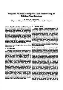
The compression scheme described below reduces the number of nodes in the transaction tree and allows further grouping of transactions that share some common items. A complete prefix tree will have many identical subtrees in it. In Figure 4a, we can see three identical subtrees st1, st2, and st3. Building a complete prefix tree will need a large amount of memory, and so we propose a method to compress the tree by storing information of identical subtrees together. For example, we can compress the full

prefix tree in Figure 4a containing 16 nodes to the tree in Figure 4b that has only 8 nodes, by storing some additional information at the nodes of the smaller tree. Given a set of n items, a prefix tree would have a maximum of 2n nodes. The corresponding compressed tree will contain a maximum of 2n-1 nodes, which is half the maximum for a full tree. In practice, the number of nodes for a transaction database will have to be far less than the maximum for the problem of frequent item set discovery to be tractable. Root

1

3

2

2

3

4

3

4

4

st1

4

3

4

4

4

st2

The paths from the root to various nodes correspond to the transactions to be traversed during mining. So compressing the prefix tree as described above can improve performance of the mining process, by grouping transactions that share common items.

3.1.2

The ITL data structure described in Section 2 is modified to take advantage of the compression achieved using the new transaction tree described above. Additional information is attached to each row of TransLink, indicating the count of transactions that have different subsets of items. A row in the modified TransLink represents a group of transactions along with a count of occurrences of each transaction of the group in the database. This contrasts with TransLink rows in the basic ITL data structure where a row represents only a single transaction. The modified ITL for the sample database is shown in Figure 6. It is described in Example 1 below.

st3

4

3.2 (a) Identical Subtrees in a Prefix tree 1 0 1 1 2 0 1 12 1 1 2 3 0 1 123 1 1 23 2 1 3

4 0 1 2 3

Modified ITL

1 1 1 1

3 0 1 13

Level 0 4

Level 1 0 1 14

4 0 1 124 4 0 1 134 1 1 24

1234 234 34 4

Level 2

Level 3

(b) Compressing the Prefix Tree Figure 4: Prefix Tree Compression In the compressed tree, we need to record the information from the pruned nodes of the complete tree. To keep the count of transactions with different item subsets, a count entry for each subset is recorded. Each count entry has two fields: the level of the starting item of the subset and the count. For example, in Figure 4b, at node 3 in the leftmost branch of the tree, there are three entries: (0,1), (1,1) and (2,1). The entry (0,1) means there is one transaction with items starting at level 0 along the path from the root of the tree to this node; it corresponds to the item set 123. The next entry (1,1) means there is one transaction with items starting at level 1 along the path from the root of the tree to this node, giving item set as 23. Similarly, (2,1) means one transaction with item 3. In this example, we have assumed the transaction count to be one at every node of the transaction tree in Figure 4a. The doted rectangles show the item sets corresponding to the nodes in the compressed tree of Figure 4b, for illustration (they are not part of the data structure).

CT-ITL Algorithm

There are four steps in the CT-ITL algorithm as follows: 1. Identify the 1-frequent item sets and initialise the ItemTable: To mine frequent item sets only 1-freq items will be needed because of the anti-monotone property of frequent sets. In this step, the transaction database is scanned to identify all 1-freq items and they are put in ItemTable. To support the compression scheme that will be used in the second step, all entries in the ItemTable are sorted in ascending order of their frequency and the items assigned new identifiers from an ascending sequence of integers. 2. Construct the compressed transaction tree: Using the output of the first step, only the 1-freq items are read from the transaction database. These items are assigned new item identifiers and the transactions inserted into the compressed transaction tree. Each node of the tree will contain a 1-freq item and a set of counts indicating the number of transactions that contain the subsets of items in the path from the root as described in Section 2. 3. Construct ITL: In this step, we traverse the transaction tree to construct the ItemTable and TransLink. 4. Mine Frequent Item Sets: All the frequent item sets of two or more items will be mined in this step using a recursive function described further in this section. The algorithm of CT-ITL is given in Figure 8. The operation of CT-ITL algorithm is illustrated by the following example. Example 1. Let the table in Figure 1 be the transaction database and suppose the user wants to get the Frequent Item sets with a minimum support of 2 transactions. In Step 1, all transactions in the database are read to identify the frequent items. For each item in a transaction, the existence of the item in the ItemTable is checked. If the item is not present in the ItemTable, it is entered with an initial count of 1; otherwise the count of the item is incremented. On completing the database scan, the 1-

frequent item sets can be identified in the ItemTable as {1, 3, 4, 5, 7}. On finishing the reading of all transactions, the entries in the ItemTable will be sorted in ascending order of item frequency. The item-ids are then mapped to an ascending sequence of integers shown as the index row in Table 1. The index entries now represent the set of new item-ids. Index 1 2 3 4 5 Item 7 5 3 1 4 Count 2 3 4 4 5

Table 1: Sorting and Mapping 1-Freq Items In Step 2, only 1-freq items are read from the database and each transaction that contain these items will be inserted into the tree using the mapping in Table 1. For example, item 7 will be mapped to 1 in the tree, 5 mapped to 2, and so on. The result of this step is shown in Figure 5. For comparison, Figure 2b shows the transaction tree with original item identifiers and without compression. It has 12 nodes while the compressed tree has only 8 nodes. 0 0 1

1

In Step 3, the TransLink attached to the ItemTable is constructed by traversing the tree using the depth first search algorithm. Conceptually, each node in the tree that has transaction count greater than zero need to be mapped to an entry in the TransLink. The tree in Figure 5 has only three such nodes, which means that there will be three entries in the TransLink. The nonzero entries of these nodes are attached to the corresponding row in TransLink. Figure 6 shows the result of Step 3 for the sample database. Transaction group t1 in the TransLink is the result of mapping the node of item 5 at the leftmost branch of the tree. The non-zero entries in that node are represented in t1. So t1 represents the transaction 2345 (original item ids 5314) that occurs once and 345 (original ids 314) that occurs twice in the database. In the implementation of modified ITL, the count entries at each row are stored in an array and so the array index is not stored explicitly. The doted rectangles that show the index at each row, is only for illustration and not part of the data structure.

Level 0 ITEMTABLE

0 0 12 1 0 2 2

Level 1

Count TRANSLINK

0 0 123 1 0 423 2 0 3

0 1 2 3 0 1 2 3 4

0 1 2 0 0

0 0 0 0

1234 4 234 34 4

12345 5 2345 345 45 5

3

0 0 124 4 1 0 24

0 1 1235 5 1 0 235 2 0 35

Index 1 2 3 4 5 Item 7 5 3 1 4 Count 2 3 4 4 5

t1

2 3 4 5

Level 2

Level 3 5 0 1 1245 1 0 245

11 2 21

t2

1 2 3 5

1 1

t3

1 2 4 5

1 1

Figure 6: The Modified ITL

Level 4

Figure 5: Compressed transaction tree for the sample database As described in Section 3.1.1, each node of the tree has additional entries to keep the count of transactions represented by the node. For example, the entry (0,0) at the leaf node of the leftmost branch of the tree represents item set 12345 that has no occurrence in the database. The first 0 indicates that the item set starts at level 0 in the tree which makes 1 its first item. The second number (which is also 0) indicates that no transaction in the database has this item set. Similarly, the entry (1,1) means there is one transaction with item set 2345 and (2,2) means there are two transactions with item set 345. In the implementation of the tree, the counts at each node are stored in an array so that the level for an entry is the array index, which is not stored explicitly. As mentioned before, the doted rectangles that show different item sets at a node are not part of the data structure.

Prefix TempList (count) 1 2 (2), 3 (1), 4 (1), 5 (2) 1 2 3 (1), 4 (1), 5(2) 2 3 (2), 4 (2), 5 (3) 2 3 4 (1), 5 (2) 2 4 5 (2) 3 4 (3), 5 (4) 3 4 5 (3) 4 5 (4) 5 None

Freq-Itemset (count) 1 (2), 1 2 (2), 1 5 (2) 1 2 5 (2) 2 (3), 2 3 (2), 2 4 (2), 2 5 (3) 2 3 5 (2) 2 4 5 (2) 3 (4), 3 4 (3), 3 5 (4) 3 4 5 (3) 4 (4), 4 5 (4) 5 (5)

Figure 7: Mining Frequent Item Sets Recursively (support of the pattern shown in brackets) In the last Step, each item in the ItemTable is used as a starting point to mine all longer frequent item sets for which it is a prefix. For example, starting with item 1, the vertical link is followed to get all other items that occur together with item 1 and the count of each item is accumulated. These items and their support count are registered in a simple table named TempList (see Figure 7) together with an associated list of {tid, count} (see Figure 9). As seen in the TempList of Figure 7, for prefix 1, we have items {2, 5} that are frequent (having count ≥ 2). Generating the frequent patterns in this step involves

simply concatenating the prefix with each frequent-item. For example, the frequent item sets for this step are 1 2 (2), and 1 5 (2) where the support of each pattern is given in parenthesis. /* Input: database */ /* Output: 1-freq item sets */ Procedure GetOneFreq For all transactions in the DB For all items in transaction If item in ItemTable Increment count of item Else Insert item with count = 1 End If End For End For /* Input: database */ /* Output: transaction tree */ Procedure Construct_Tree For all transactions in the DB For all items in transaction If count(item) in ItemTable ≥ min_sup Insert the item into the tree End If End For End For /* Input : transaction tree */ /* Output: ITL */ Procedure Construct_ITL For each path in the tree traversed by depth first search Map the path as an entry in TransLink Attach the count entries of the path Establish links in TransLink to previous occurrences of each item End For /* Input : ITL */ /* Output: Frequent Item Sets */ Procedure MineFI For all xŒItemTable where count(x)≥min_sup Add x to the set of Freq-ItemSets Prepare and fill tempList for x For all yŒtempList where count(y) ≥ min_sup Add xy to the set of Freq-ItemSets For all zŒtempList after y where count(z) ≥ min_sup RecMine(xy,z) EndFor End For End For Procedure RecMine(prefix, testItem) tlp:= tid-count-list of prefix tli:= tid-count-list of testItem tl_current:= Intersect(tlp,tli) If size(tl_current) ≥ min_sup new_prefix:= prefix + testItem Add new_prefix to the set of FreqItemSets For all zŒtempList after testItem where count(z) ≥ min_sup RecMine(new_prefix, z) End For End If

Figure 8: CT-ITL Algorithm

After generating the 2-frequent-item sets for prefix 1, the associated tid-count lists of items in the TempList, are used to recursively generate frequent sets of 3 items, 4 items and so on. For example, the tid list of 1 2 is intersected with tid list of 1 5 to generate the frequent item set 1 2 5. At the end of recursive calls with item 1, all frequent item sets that contains item 1 would be generated: 1 (2), 1 2 (2), 1 5 (2), 1 2 5 (2). In the next sequence, item 2 will be used to generate all frequent item sets that contain item 2 but does not contain item 1. Then item 3 will be used to generate all frequent item sets that contain item 3 but does not contain items 1 and 2. Before writing the output, the frequent item sets are mapped to the real item identifiers using the ItemTable: 7 (2), 57 (2), 457 (2), 47 (2), etc. in the example, where the support counts are shown in parenthesis.

3.3

Tid-Count Intersection

As discussed in the previous sub section, the (tid, count) lists of items are recorded in the TempList. This method significantly improves the mining process by avoiding repeated traversals of TransLink. The initial tid-count-list is built by traversing the vertical link in the TransLink. For example, during the mining of all frequent item sets beginning with item 1, a TempList entry as shown in Figure 9a is built. Each item in the TempList will have the total count (shown in brackets) of the item’s occurrences with the prefix item and also the tid-countlist of the item. 1

prefix

2 (2) 2 3

1 1

3 (1) 2

1

4 (1) 3

1

5 (2) 2 3

1 1

tid count (a) With tid and count as separate entries 1

2 (2) 11 16

3 (1) 11

4 (1) 16

5 (2) 11 16

(b) With tid and count as a single entry Figure 9: Tid-Count-List If the total count is greater than or equal to the supportthreshold, then the concatenation of the prefix with the item is a frequent item set. In Figure 9, the frequent item sets are 1 2 (2) and 1 5 (2). Mining item sets 1 2 3 after generating frequent item set 1 2 is basically similar to running a merge-sort program between tid-count-lists of items 2 and 3. Similarly, we can use the tid-count-lists of item 2 with that of items 4 or 5 to mine item sets 1 2 4 or 1 2 5. In the implementation, keeping the tid and count as separate entries in the list affects the performance adversely, so we combine the tid and count values into a single field using the following formula: tid_count = (tid * max_count) + item_count

Max_count is the maximum occurrence of all items in the ItemTable. In the example, max_count is 5 since 5 is the highest frequency (item 4). In the TempList, tid 2 with count 1 will be stored as 11 (2 * 5 + 1), tid 3 as 16. count = tid_count MOD max_count To determine the count of each group of transactions we can use the above formula, e.g., 11 mod 5 = 1, 16 mod 5 = 1. Using this method, we can simplify the tid-count-list (as shown in Figure 9b). Implementing this method saves space in memory and improves performance of tid-count intersection.

4

Performance Study

In this section, the performance evaluation of CT-ITL is presented. The fastest available implementation of Apriori was chosen to represent the candidate generationand-test approach in our comparisons. Similarly OP is currently the fastest available program based on the pattern growth approach. Eclat is used in our evaluations because its implementation is based on tid-intersection of frequent item sets. TreeITL-Mine is a variant of our algorithm that uses an uncompressed tree for transaction grouping. It has been used to study the impact of the compressed tree on the overall performance of our algorithm. Dataset # of Trans # of items Mushroom 8,124 119 Chess 3,196 75 BMS-Web-View1 59,602 497 Connect-4 67,557 129 Pumsb* 49,046 2,087

Avg Trans Size 23 37 2.5 43 50

Table 2. Test Dataset Characteristics Dataset

Support

Mushroom

25 20 15 10 5 90 80 70 60 50 0.1 0.09 0.08 0.07 0.06 95 90 85 80 75 70 60 50 40 30

Chess

BMS Web View1

Connect-4

Pumsb*

1-freq item 35 43 48 56 73 13 19 24 34 37 343 350 352 360 368 17 21 25 28 30 9 14 27 46 59

Frequent Item Sets 5545 53583 98575 574431 3755511 622 8227 48731 254944 1272932 3991 5786 10286 27403 461521 2201 27127 142127 533975 1585551 29 167 679 27354 432482

TransLink Entries 867 1889 3067 5339 7450 39 193 469 2081 2969 17847 17903 17918 17973 18031 17 32 70 123 171 62 471 3183 10505 18176

Table 3. Number of Frequent Item Sets Generated All the programs are written in Microsoft Visual C++ 6.0. All the testing was performed on an 866MHz Pentium III PC, 512 MB RAM, 30 GB HD running Microsoft Windows 2000. In this paper, the runtime includes both CPU time and I/O time. Several datasets were used to test the performance including Mushroom, Chess, Connect-4, Pumsb* and BMS-Web-View1. The Mushroom dataset describes the characteristics of various species of mushrooms. The Chess dataset is derived from the steps of Chess games. In Connect-4, each transaction contains 8-ply positions in the game of connect-4 where no player has won yet and the next move is not forced. All of them were downloaded from Irvine Machine Learning Database Repository. Pumsb* contains census data from PUMS (Public Use Microdata Samples). Each transaction represents the answers to a census questionnaire, including the age, tax-filing status, marital status, income, sex, veteran status, and location of residence of the respondent. In Pumsb* all items with 80% or more support in the original PUMS data set are deleted. BMSWeb-View1 representing a real life dataset comes from a small dot-com company called Gazelle.com, a legwear and legcare retailer, which no longer exists. It contains several months’ worth of clickstream data from an ecommerce web site. Table 2 shows the characteristics of each dataset. Dataset Sup Mushroom 25 20 15 10 5 Chess 90 80 70 60 50 BMS 0.1 Web 0.09 View1 0.08 0.07 0.06 Connect-4 95 90 85 80 75 Pumsb* 70 60 50 40 30

Ranking CT-ITL > Eclat > OP > TreeITL-Mine > Apriori OP > Eclat > CT-ITL > TreeITL-Mine > Apriori OP > Eclat > CT-ITL > TreeITL-Mine > Apriori OP > Eclat > CT-ITL > TreeITL-Mine > Apriori OP > Eclat > CT-ITL > TreeITL-Mine > Apriori CT-ITL > Eclat > OP > TreeITL-Mine > Apriori CT-ITL > Eclat > OP > TreeITL-Mine > Apriori OP > Eclat > CT-ITL > TreeITL-Mine > Apriori OP > Eclat > CT-ITL > TreeITL-Mine > Apriori OP > Eclat > CT-ITL > Apriori > TreeITL-Mine OP > Apriori > CT-ITL > TreeITL-Mine > Eclat OP > Apriori > CT-ITL > TreeITL-Mine > Eclat OP > Apriori > CT-ITL > TreeITL-Mine > Eclat OP > CT-ITL > Apriori > TreeITL-Mine > Eclat OP > CT-ITL > TreeITL-Mine > Apriori > Eclat CT-ITL > Eclat > OP > TreeITL-Mine > Apriori CT-ITL > OP > Eclat > TreeITL-Mine > Apriori CT-ITL > OP > Eclat > TreeITL-Mine > Apriori CT-ITL > OP >Eclat > TreeITL-Mine > Apriori OP > CT-ITL > Eclat > TreeITL-Mine > Apriori TreeITL-Mine > CT-ITL > Apriori > OP > Eclat CT-ITL > TreeITL-Mine > OP > Apriori > Eclat CT-ITL > TreeITL-Mine > OP > Apriori > Eclat OP > CT-ITL > Eclat > TreeITL-Mine > Apriori OP > Eclat > CT-ITL > TreeITL-Mine > Apriori

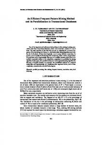
Table 4. Ranking of Algorithms Performance comparisons of CT-ITL, TreeITL-Mine, Apriori, Eclat and OP on the various datasets are shown in Figures 10 and 11. All the charts use a logarithmic scale along the y-axis. The ranking of algorithms vary on

the different datasets and support levels we used (see Table 4). CT-ITL outperforms all other algorithms on Pumsb* (support 50-60), Connect-4 (support 80-95), Chess (support 80-90) and Mushroom (support 25). CT-ITL performs better than other algorithms at high support levels. As the support threshold gets lower and the number of frequent item sets generated is significantly higher (see Table 3), the performance of OP improves.

In Pumsb*, as with Connect-4, the reduction in number of TransLink entries by compressing transactions is very significant at support levels of 50-60 which helps CT-ITL perform better than other algorithms. On Chess, CT-ITL outperforms other algorithms at supports 80 and 90 and it is not much different from OP at support 70. From support 70 to support 60, the number of TransLink entries increased significantly from 469 to 2,081 while the number of transactions is 3,196 at 60% support. This explains the narrowing gap between OP and CT-ITL at the lower support levels. 100

CHESS Runtime (seconds)

Runtime (seconds)

1000 100 10 1 0.1 50

60

70

80

BMS-WEB-VIEW1 10

1

0.1 0.06

90

Support Threshold (%)

Runtime (seconds)

Runtime (seconds)

100 10 1 0.1 15

20

1000 100 10 1

25

75

80

85

90

95

Support Threshold (%)

TreeITL-Mine

Figure 10. Performance comparisons of Apriori, TreeITL-Mine, OP, CT-ITL and Eclat on Chess and Mushroom In BMS-Web-View1, a sparse dataset with average transaction size of only 2.5, CT-ITL outperforms TreeITL-Mine and Eclat. At support of 0.07 and 0.06, CT-ITL performed better than Apriori, TreeITL-Mine and Eclat. On Connect-4, CT-ITL outperforms other algorithms at most of the support levels we used. This is because the number of TransLink entries is very low compared to the number of transactions in the original database. For example, at support 95, the number of entries in TransLink is only 17 while the original number of transactions is 67,557 (see Table 3). Since Apriori does not have any compression scheme, it performs poorly on a dense data set like Connect-4. As seen in Table 3, the number of frequent patterns in this data set increases dramatically from 2,201 at support 95 to 1,585,551 at support 75.

10000

Runtime (seconds)

OP CT-ITL

0.1

CONNECT-4

10000

Support Threshold (%)

Apriori Eclat

0.09

100000

MUSHROOM

10

0.08

Support Threshold (%)

1000

5

0.07

PUMSB* 1000 100 10 1 30

40

50

60

70

Support Threshold (%)

Apriori Eclat

OP CT-ITL

TreeITL-Mine

Figure 11. Performance comparisons of Apriori, TreeITL-Mine, OP, CT-ITL and Eclat on BMS-Web-View1, Connect-4 and Pumsb* Mushroom is also a very dense dataset like Connect-4. The number of frequent item sets increases significantly

from 5,545 at 25% support to 3,755,511 at 5% support. At 25% support, the number of TransLink entries generated is 867 (original number of transactions 8,124). CT-ITL outperforms other algorithms at this support level. At 20% support, number of TransLink entries becomes 1,889 (more than twice compared to 20% support), and keep increasing to 7,450 at 5% support and so the degree of compression is not very good at this level. However CT-ITL performed better than Apriori and TreeITL-Mine at all support levels we used for this dataset.

5

3.

Discussion

In this section, we discuss the similarities and differences between CT-ITL and other comparable algorithms. We also consider the problem of mining very large databases and the support for interactive mining.

5.1

2.

4.

Comparison with Other Algorithms

We compare CT-ITL with a few well-known algorithms that have similar features. In the following, we highlight the significant differences between our algorithm and others: FP-Growth. The FP-Growth algorithm builds an FP-Tree based on the prefix tree concept and uses it during the whole mining process (Han, Pei and Yin 2000). We have refined the prefix tree structure by reducing the number of nodes and used the compressed tree for grouping transactions. In order to reduce the number of column traversals (in the conceptual binary table of Section 2) using tid-intersection, the tree is mapped to ITL data structure. The cost of mapping the tree to ITL is justified by the performance gain obtained in the last step of mining frequent item sets. FP-Growth uses item frequency descending order in building the FP-Tree. For most data sets, descending order usually creates fewer nodes compared to ascending order. However, we found in our experiments that descending order creates more TransLink entries compared to the ascending order, for the typical data sets used. It was also found that fewer the entries in ITL, faster the performance of CT-ITL. Eclat. Tid-intersection used by Zaki creates a tid-list of all transactions in which an item occurs (Zaki 2000). In our algorithm, each tid in the tid-list represents a group of transactions and a count of transactions is noted for each group. The tid and count are used together in tid-count intersection. The tid-count lists are shorter because of transaction grouping and therefore perform faster intersections. H - M i n e . In the mining of frequent item sets after constructing the ITL, our algorithm may appear similar to H-Mine but there are significant differences between the two as given below: 1. In the ITL data structure of CT-ITL, each row is a group of transactions while in H-struct, each row represents a single transaction in the database. Grouping the transactions significantly reduces the number of rows in ITL compared to H-struct.

5.

After the ITL data structure is constructed, it remains unchanged while mining all of the frequent patterns. In H-Mine, the pointers in the H-struct need to be continually re-adjusted during the extraction of frequent patterns and so needs additional computation. CT-ITL uses a simple temporary table called TempList during the recursive extraction of frequent patterns. CT-ITL need to store in the TempList only the information for the current recursive call which will be deleted from the memory if the recursive call backtracks to the upper level. H-Mine builds a series of header tables linked to the H-struct and it needs to change pointers to create or re-arrange queues for each recursive call. H-Mine needs to traverse from the beginning of each transaction to check whether a pattern exists in it. We use tid-count-intersection that is basically a mergesort algorithm, for extending frequent patterns. Thus we mostly avoid the expensive horizontal traversals of transactions. Depending on the characteristics of the dataset, using a compressed prefix tree to group transactions can make the number of ITL entries to be traversed by CT-ITL much smaller than for H-Mine.

OpportuneProject (OP). OP is currently the fastest available program based on pattern growth approach. OP is an adaptive algorithm that can choose between an array and a tree to represent the transactions in the memory. It can also use different methods of projecting the database while generating the frequent item sets. However, OP is essentially a combination of FP-Growth and H-Mine. As discussed in Section 4, our compression method makes CT-ITL perform better than OP on several typical datasets and support levels.

5.2

Mining Large Databases

Using the compressed tree and the modified ITL, mining can be carried out efficiently even for relatively large databases for which the tree containing 1-frequent items fits into main memory. However, we cannot assume that the tree will always fit in the memory for very large databases, even with significant compression. The extension of this algorithm by using the idea of partitioning the tree is currently in progress.

5.3

Interactive Mining

Our algorithm supports more efficient interactive mining, where the user may experiment with different values of minimum support levels. Using the constructed ItemTable and TransLink in the memory, if the user wants to change the value of support threshold (as long as the support level is higher than previous), there is no need to re-read the transaction database.

6

Conclusion

In this paper, we have presented a new algorithm called CT-ITL for discovering complete frequent item sets. We use the Item-Trans Link (ITL) data structure that combines the benefits of both horizontal and vertical data

layouts for association rule mining. We modified the basic ITL so that groups of transactions can be stored together instead of recording each individual transaction separately. A prefix-tree is used to form transaction groups and a new method has been developed to compress the tree for efficient use of memory. The performance of CT-ITL was compared against TreeITLMine, Apriori, Eclat and OP on various datasets and the results showed that when the compression ratio is significant CT-ITL outperformed all others. We discussed the results in detail and pointed out the strengths and weaknesses of our algorithm. We have assumed in this paper that the ItemTable, TransLink and the compressed transaction tree will fit into main memory. However, this assumption will not apply for huge databases. To extend this algorithm for very large databases, we plan to partition the tree to fit in available memory. This work is currently in progress. Several researchers have investigated the use of constraints to reduce the size of frequent item sets and to allow greater user focus in the mining process (Pei, Han and Lakshmanan 2001). To make the mining process more efficient, the main idea is to push the constraints deep inside the algorithm. It is planned to integrate the processing of constraints into CT-ITL.

7

Acknowledgement

We are grateful to Junqiang Liu for providing us the OpportuneProject program and to Christian Borgelt for making available his implementations of Apriori and Eclat algorithms.

8

References

AGARWAL, R., AGGARWAL, C. and PRASAD, V.V.V. (2000): A Tree Projection Algorithm for Generation of Frequent Itemsets. Journal of Parallel and Distributed Computing (Special Issue on High Performance Data Mining). AGRAWAL, R., IMIELINSKI, T. and SWAMI, A. (1993): Mining Association Rules between Sets of Items in Large Databases. Proc. of ACM SIGMOD, Washington DC, 22:207-216, ACM Press. AGRAWAL, R. and SRIKANT, R. (1994): Fast Algorithms for Mining Association Rules. Proc. of the 20th International Conference on Very Large Data Bases, Santiago, Chile, 487-499. GOPALAN, R.P. and SUCAHYO, Y.G. (2002): TreeITL-Mine: Mining Frequent Itemsets Using Pattern Growth, Tid Intersection and Prefix Tree. Proc. of 15th Australian Joint Conference on Artificial Intelligence, Canberra, Australia.. HAN, J., PEI, J. and YIN, Y. (2000): Mining Frequent Patterns without Candidate Generation. Proc. of ACM SIGMOD, Dallas, TX. LIU, J., PAN, Y., WANG, K. and HAN, J. (2002): Mining Frequent Item Sets by Opportunistic Projection. Proc. of ACM SIGKDD, Edmonton, Alberta, Canada.

PEI, J., HAN, J. and LAKSHMANAN, L.V.S. (2001): Mining Frequent Itemsets with Convertible Constraints. Proc. of 17th International Conference on Data Engineering, Heidelberg, Germany. PEI, J., HAN, J., LU, H., NISHIO, S., TANG, S. and YANG, D. (2001): H-Mine: Hyper-Structure Mining of Frequent Patterns in Large Databases. Proc. of the IEEE ICDM, San Jose, California. SHENOY, P., HARITSA, J.R., SUDARSHAN, S., BHALOTIA, G., BAWA, M. and SHAH, D. (2000): Turbo-charging Vertical Mining of Large Databases. Proc. of ACM SIGMOD, Dallas, TX USA, 22-33. ZAKI, M.J. (2000): Scalable Algorithms for Association Mining. IEEE Transactions on Knowledge and Data Engineering 12(3):372-390. ZAKI, M.J. and GOUDA, K. (2001): Fast Vertical Mining Using Diffsets. RPI Technical Report 01-1. Rensselaer Polytechnic Institute, Troy, NY 12180 USA. New York.