Simple Algorithms for Frequent Item Set Mining - Semantic Scholar

Simple Algorithms for Frequent Item Set Mining Christian Borgelt European Center for Soft Computing c/ Gonzalo Guti´errez Quir´os s/n, 33600 Mieres, Asturias, Spain [email protected]

Abstract. In this paper I introduce SaM, a split and merge algorithm for frequent item set mining. Its core advantages are its extremely simple data structure and processing scheme, which not only make it quite easy to implement, but also very convenient to execute on external storage, thus rendering it a highly useful method if the transaction database to mine cannot be loaded into main memory. Furthermore, I review RElim (an algorithm I proposed in an earlier paper and improved in the meantime) and discuss different optimization options for both SaM and RElim. Finally, I present experiments comparing SaM and RElim with classical frequent item set mining algorithms (like Apriori, Eclat and FP-growth).

1

Introduction

It is hardly an exaggeration to say that the popular research area of data mining was started by the tasks of frequent item set mining and association rule induction. At the very least, these tasks have a strong and long-standing tradition in data mining and knowledge discovery in databases and triggered an abundance of publications in data mining conferences and journals. The huge research efforts devoted to these tasks have led to a variety of sophisticated and efficient algorithms to find frequent item sets. Among the best-known approaches are Apriori [1, 2], Eclat [17] and FP-growth [11]. Nevertheless, there is still room for improvement: while Eclat, which is the simplest of the mentioned algorithms, can be relatively slow on some data sets (compared to other algorithms, see the experimental results reported in Section 5), FP-growth, which is usually the fastest algorithm, employs a sophisticated and rather complex data structure and thus requires to load the transaction database into main memory. Hence a simpler processing scheme, which maintains efficiency, is desirable. Other lines of improvement include filtering found frequent item sets and association rules (see, e.g., [22, 23]), identifying temporal changes in discovered patterns (see, e.g., [4, 5]), and discovering fault-tolerant or approximate frequent item sets (see, e.g., [9, 14, 21]). In this paper I introduce SaM, a split and merge algorithm for frequent item set mining. Its core advantages are its extremely simple data structure and processing scheme, which not only make it very easy to implement, but also convenient to execute on external storage, thus rendering it a highly useful method if the transaction database to mine cannot be loaded into main memory. Furthermore, I review RElim, an also very simple algorithm, which I proposed in an earlier paper [8] and which can be seen as a precursor of SaM. In addition, I study different ways of optimizing RElim and SaM, while preserving, as far as possible, the simplicity of their basic processing schemes.

The rest of this paper is structured as follows: Section 2 briefly reviews the task of frequent item set mining and especially the basic divide-and-conquer scheme underlying many frequent item set mining algorithms. In Section 3 I present my new SaM (Split and Merge) algorithm for frequent item set mining, while in Section 4 I review its precursor, the RElim algorithm, which I proposed in an earlier paper [8]. In Section 5 the basic versions of both SaM and RElim are compared experimentally to classical frequent item set mining algorithms like Apriori, Eclat, and FP-growth, and the results are analyzed. Based on this analysis, I suggest in Section 6 several optimization options for both SaM and RElim and then present the corresponding experimental results in Section 7. Finally, in Section 8, I draw conclusions from the discussion.

2

Frequent Item Set Mining

Frequent item set mining is a data analysis method, which was originally developed for market basket analysis and which aims at finding regularities in the shopping behavior of the customers of supermarkets, mail-order companies and online shops. In particular, it tries to identify sets of products that are frequently bought together. Once identified, such sets of associated products may be used to optimize the organization of the offered products on the shelves of a supermarket or the pages of a mail-order catalog or web shop, or may give hints which products may conveniently be bundled. Formally, the task of frequent item set mining can be described as follows: we are given a set B of items, called the item base, and a database T of transactions. Each item represents a product, and the item base represents the set of all products offered by a store. The term item set refers to any subset of the item base B. Each transaction is an item set and represents a set of products that has been bought by an actual customer. Since two or even more customers may have bought the exact same set of products, the total of all transactions must be represented as a vector, a bag or a multiset, since in a simple set each transaction could occur at most once.1 Note that the item base B is usually not given explicitly, but only implicitly as the union of all transactions. The support sT (I) of an item set I ⊆ B is the number of transactions in the database T , it is contained in. Given a user-specified minimum support smin ∈ IN, an item set I is called frequent in T iff sT (I) ≥ smin . The goal of frequent item set mining is to identify all item sets I ⊆ B that are frequent in a given transaction database T . Note that the task of frequent item set mining may also be defined with a relative minimum support, which is the fraction of transactions in T that must contain an item set I in order to make I frequent. However, this alternative definition is obviously equivalent. A standard approach to find all frequent item sets w.r.t. a given database T and support threshold smin , which is adopted by basically all frequent item set mining algorithms (except those of the Apriori family), is a depth-first search in the subset lattice of the item base B. Viewed properly, this approach can be interpreted as a simple divideand-conquer scheme. For some chosen item i, the problem to find all frequent item sets is split into two subproblems: (1) find all frequent item sets containing the item i and (2) find all frequent item sets not containing the item i. Each subproblem is then further 1

Alternatively, each transaction may be enhanced by a unique transaction identifier, and these enhanced transactions may then be combined in a simple set.

divided based on another item j: find all frequent item sets containing (1.1) both items i and j, (1.2) item i, but not j, (2.1) item j, but not i, (2.2) neither item i nor j, and so on. All subproblems that occur in this divide-and-conquer recursion can be defined by a conditional transaction database and a prefix. The prefix is a set of items that has to be added to all frequent item sets that are discovered in the conditional database. Formally, all subproblems are tuples S = (C, P ), where C is a conditional database and P ⊆ B is a prefix. The initial problem, with which the recursion is started, is S = (T, ∅), where T is the transaction database to mine and the prefix is empty. A subproblem S0 = (C0 , P0 ) is processed as follows: Choose an item i ∈ B0 , where B0 is the set of items occurring in C0 . This choice is arbitrary, but usually follows some predefined order of the items. If sC0 (i) ≥ smin , then report the item set P0 ∪ {i} as frequent with the support sC0 (i), and form the subproblem S1 = (C1 , P1 ) with P1 = P0 ∪ {i}. The conditional database C1 comprises all transactions in C0 that contain the item i, but with the item i removed. This also implies that transactions that contain no other item than i are entirely removed: no empty transactions are ever kept. If C1 is not empty, process S1 recursively. In any case (that is, regardless of whether sC0 (i) ≥ smin or not), form the subproblem S2 = (C2 , P2 ), where P2 = P0 and the conditional database C2 comprises all transactions in C0 (including those that do not contain the item i), but again with the item i removed. If C2 is not empty, process S2 recursively. Eclat, FP-growth, RElim and several other frequent item set mining algorithms rely on this basic scheme, but differ in how they represent the conditional databases. The main approaches are horizontal and vertical representations. In a horizontal representation, the database is stored as a list (or array) of transactions, each of which is a list (or array) of the items contained in it. In a vertical representation, a database is represented by first referring with a list (or array) to the different items. For each item a list (or array) of identifiers is stored, which indicate the transactions that contain the item. However, this distinction is not pure, since there are many algorithms that use a combination of the two forms of representing a database. For example, while Eclat uses a purely vertical representation, FP-growth combines in its FP-tree structure a vertical representation (links between branches) and a (compressed) horizontal representation (prefix tree of transactions). RElim uses basically a horizontal representation, but groups transactions w.r.t. their leading item, which is, at least partially, a vertical representation. The SaM algorithm presented in the next section is, to the best of my knowledge, the first frequent item set mining algorithm that is based on the general processing scheme outlined above and uses a purely horizontal representation.2 The basic processing scheme can easily be improved with so-called perfect extension pruning, which relies on the following simple idea: given an item set I, an item i∈ / I is called a perfect extension of I, iff I and I ∪ {i} have the same support, that is, if i is contained in all transactions containing I. Perfect extensions have the following properties: (1) if the item i is a perfect extension of an item set I, then it is also a perfect extension of any item set J ⊇ I as long as i ∈ / J and (2) if I is a frequent item set and K is the set of all perfect extensions of I, then all sets I ∪ J with J ∈ 2K (where 2K denotes the power set of K) are also frequent and have the same support as I. 2

Note that Apriori, which also uses a purely horizontal representation, relies on a different processing scheme, since it traverses the subset lattice level-wise rather than depth-first.

1j a d acde bd bcd bc abd bde bcde bc abd

2j e: a: c: b: d:

3 4 5 8 8

3j a d eacd bd cbd cb abd ebd ecbd cb abd

4j e a c d ecbd ebd abd abd ad cbd cb cb bd

5j 1 1

e a c d e c b d

1

e b d a b d a d

1

c b d

2

c b b d

1 2

1

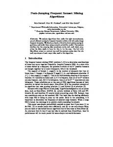
Fig. 1. The example database: original form (1), item frequencies (2), transactions with sorted items (3), lexicographically sorted transactions (4), and the data structure used by SaM (5).

These properties can be exploited by collecting in the recursion not only prefix items, but also, in a third element of a subproblem description, perfect extension items. Once identified, perfect extension items are no longer processed in the recursion, but are only used to generate all supersets of the prefix that have the same support. Depending on the data set, this can lead to a considerable speed-up. It should be clear that this optimization can, in principle, be applied in all frequent item set mining algorithms.

3

A Split and Merge Algorithm

The SaM (Split and Merge) algorithm I introduce in this paper can be seen as a simplification of the already fairly simple RElim (Recursive Elimination) algorithm, which I proposed in [8]. While RElim represents a (conditional) database by storing one transaction list for each item (partially vertical representation), the split and merge algorithm presented here employs only a single transaction list (purely horizontal representation), stored as an array. This array is processed with a simple split and merge scheme, which computes a conditional database, processes this conditional database recursively, and finally eliminates the split item from the original (conditional) database. SaM preprocesses a given transaction database in a way that is very similar to the preprocessing used by many other frequent item set mining algorithms. The steps are illustrated in Figure 1 for a simple example transaction database. Step 1 shows the transaction database in its original form. In step 2 the frequencies of individual items are determined from this input in order to be able to discard infrequent items immediately. If we assume a minimum support of three transactions for our example, there are no infrequent items, so all items are kept. In step 3 the (frequent) items in each transaction are sorted according to their frequency in the transaction database, since it is well known that processing the items in the order of increasing frequency usually leads to the shortest execution times. In step 4 the transactions are sorted lexicographically into descending order, with item comparisons again being decided by the item frequencies, although here the item with the higher frequency precedes the item with the lower frequency. In step 5 the data structure on which SaM operates is built by combining equal transactions and setting up an array, in which each element consists of two fields: an

1 1

e a c d e c b d

split

2

e b d a b d

1

a d

1

c b d

1

2

c b b d

1

1

2

a c d a b d

1 1

a d

2

c b d

1

a b d a d

2

1

c b d

2

c b b d

1

a c d c b d

2

1

b d

1

c b b d

2 prefix e

merge

e removed

prefix e

1

a c d c b d

1

b d

1

Fig. 2. The basic operations of the SaM algorithm: split (left) and merge (right).

occurrence counter and a pointer to the sorted transaction (array of contained items). This data structure is then processed recursively to find the frequent item sets. The basic operations of the recursive processing, which follows the general depthfirst/divide-and-conquer scheme reviewed in Section 2, are illustrated in Figure 2. In the split step (see the left part of Figure 2) the given array is split w.r.t. the leading item of the first transaction (item e in our example): all array elements referring to transactions starting with this item are transferred to a new array. In this process the pointer (in)to the transaction is advanced by one item, so that the common leading item is “removed” from all transactions. Obviously, this new array represents the conditional database of the first subproblem (see Section 2), which is then processed recursively to find all frequent items sets containing the split item (provided this item is frequent). The conditional database for frequent item sets not containing this item (needed for the second subproblem, see Section 2) is obtained with a simple merge step (see the right part of Figure 2). The new array created in the split step and the rest of the original array (which refers to transactions starting with a different item) are combined with a procedure that is almost identical to one phase of the well-known mergesort algorithm. Since both arrays are obviously lexicographically sorted, a single traversal suffices to create a lexicographically sorted merged array. The only difference to a mergesort phase is that equal transactions (or transaction suffixes) are combined. That is, there is always just one instance of each transaction (suffix), while its number of occurrences is kept in the occurrence counter. In our example this results in the merged array having two elements less than the input arrays together: the transaction (suffixes) cbd and bd, which occur in both arrays, are combined and their occurrence counters are increased to 2. Note that in both the split and the merge step only the array elements (that is, the occurrence counter and the (advanced) transaction pointer) are copied to a new array. There is no need to copy the transactions themselves (that is, the item arrays), since no changes are ever made to them. (In the split step the leading item is not actually removed, but only skipped by advancing the pointer (in)to the transaction.) Hence it suffices to have one global copy of all transactions, which is merely referred to in different ways from different arrays used in the recursive processing. Note also that the merge result may be created in the array that represented the original (conditional) database, since its front elements have been cleared in the split step. In addition, the array for the split database can be reused after the recursion for the

function SaM (a: array of transactions, (∗ conditional database to process ∗) p: set of items, (∗ prefix of the conditional database a ∗) smin : int) : int (∗ minimum support of an item set ∗) var i: item; (∗ buffer for the split item ∗) s: int; (∗ support of the current split item ∗) n: int; (∗ number of found frequent item sets ∗) b, c, d: array of transactions; (∗ split result and merged database ∗) begin (∗ — split and merge recursion — ∗) n := 0; (∗ initialize the number of found item sets ∗) while a is not empty do (∗ while conditional database is not empty ∗) b := empty; s := 0; (∗ initialize split result and item support ∗) i := a[0].items[0]; (∗ get leading item of the first transaction ∗) while a is not empty and a[0].items[0] = i do (∗ and split database w.r.t. this item ∗) s := s + a[0].wgt; (∗ sum the occurrences (compute support) ∗) remove i from a[0].items; (∗ remove the split item from the transaction ∗) if a[0].items is not empty (∗ if the transaction has not become empty ∗) then remove a[0] from a and append it to b; else remove a[0] from a; end; (∗ move it to the conditional database, ∗) end; (∗ otherwise simply remove it ∗) c := b; d := empty; (∗ note split result, init. the output array ∗) while a and b are both not empty do (∗ merge split and rest of database ∗) if a[0].items > b[0].items (∗ copy lex. smaller transaction from a ∗) then remove a[0] from a and append it to d; else if a[0].items < b[0].items (∗ copy lex. smaller transaction from b ∗) then remove b[0] from b and append it to d; else b[0].wgt := b[0].wgt +a[0].wgt; (∗ sum the occurrence counters/weights ∗) remove b[0] from b and append it to d; remove a[0] from a; (∗ move combined transaction and ∗) end; (∗ delete the other, equal transaction: ∗) end; (∗ keep only one instance per transaction ∗) while a is not empty do (∗ copy the rest of the transactions in a ∗) remove a[0] from a and append it to d; end; while b is not empty do (∗ copy the rest of the transactions in b ∗) remove b[0] from b and append it to d; end; a := d; (∗ second recursion is executed by the loop ∗) if s ≥ smin then (∗ if the split item is frequent: ∗) p := p ∪ {i}; (∗ extend the prefix item set and ∗) report p with support s; (∗ report the found frequent item set ∗) n := n + 1 + SaM(c, p, smin ); (∗ process the created database recursively ∗) p := p − {i}; (∗ and sum the found frequent item sets, ∗) end; (∗ then restore the original item set prefix ∗) end; return n; (∗ return the number of frequent item sets ∗) end; (∗ function SaM() ∗) Fig. 3. Pseudo-code of the SaM algorithm. The actual C code is even shorter than this description, despite the fact that it contains additional functionality, because certain operations needed in this algorithm can be written very concisely in C (using pointer arithmetic to process arrays).

1j · · ·

3j

see Figure 1

4j e a c d ecbd ebd abd abd ad cbd cb cb bd

5j d b c a e 0 1 3 3 3

1

d

1

b d

2

b d

1

a c d

2

b

1

d

1

c b d

1

b d

Fig. 4. Preprocessing the example database for the RElim algorithm and the initial data structure.

split w.r.t. to the next item. As a consequence, each recursion step, which expands the prefix of the conditional database, only needs to allocate one new array, with a size that is limited to the size of the input array of that recursion step. This makes the algorithm not only simple in structure, but also very efficient in terms of memory consumption. Finally, note that due to the fact that only a simple array is used as the data structure, the algorithm can fairly easily be implemented to work on external storage or a (relational) database system. There is, in principle, no need to load the transactions into main memory and even the array may easily be stored as a simple (relational) table. The split operation can then be implemented as an SQL select statement, the merge operation is very similar to a join, even though it may require a more sophisticated comparison of transactions (depending on how the transactions are actually stored). Pseudo-code of the recursive procedure is shown in Figure 3. As can be seen, a single page of code is sufficient to describe the whole recursion in detail. The actual C code I developed is even shorter than this pseudo-code, despite the fact that the C code contains additional functionality (like, for example, perfect extension pruning, see Section 2), because certain operations needed in this algorithm can be written very concisely in C (especially when using pointer arithmetic to process arrays).

4

A Recursive Elimination Algorithm

The RElim (Recursive Elimination) algorithm [8] can be seen as a precursor of the SaM algorithm introduced in the preceding section. It also employs a basically horizontal transaction representation, but separates the transactions (or transaction suffixes) according to their leading item, thus introducing a vertical representation aspect. The transaction database to mine is preprocessed in essentially the same way as for the SaM algorithm (cf. Figure 1). Only the final step (step 5), in which the data structure to work on is constructed, differs: instead of listing all transactions in one array, they are grouped according to their leading item (see Figure 4 on the right). In addition, the transactions are organized as lists (at least in my implementation), even though, in principle, using arrays would also be possible. These lists are sorted descendingly w.r.t. the frequency of their associated items in the transaction database: the first list is associated with the most frequent item, the last list with the least frequent item.

d b c a e 0 1 3 3 3

1

d

d b c a 0 1 1 1

initial database

1

b d

2

b d

1

a c d

2

b

1

d

1

c b d

1

b d

d b c a 0 2 4 4

e eliminated

1

d

1

b d

1

c d

1

d

1

b d

2

b d

2

b

1

d

1

d

prefix e

1

b d

1

c d

Fig. 5. The basic operations of the RElim algorithm. The rightmost list is traversed and reassigned: once to an initially empty list array (conditional database for the prefix e, see top right) and once to the original list array (eliminating item e, see bottom left). These two databases are then both processed recursively.

Note that each transaction list contains in its header a counter for the number of transactions. For the last (rightmost) list, this counter states the support of the associated item in the represented (conditional) database. For a preceding list, however, the value of this counter may be lower than the support of the item associated with the list, because this item may also occur in transactions starting with items following it in the item order (that is, with items that occur less frequently in the transaction database). Note also that the leading item of each transaction has already been removed from all transactions, as it is implicitly represented by which list a transaction is contained in and thus need not be explicitly present. As a consequence, the counter associated with each transaction list need not be equal to the sum of the weights of the transactions in the list (even though this is the case in the example), because transactions (or transaction suffixes) that contain only the item (and thus become empty if the item is removed) are not explicitly represented by a list element, but only implicitly in the counter. The basic operations of the RElim algorithm are illustrated in Figure 5. The next item to be processed is the one associated with the last (rightmost) list (in the example this is item e). If the counter associated with the list, which states the support of the item, exceeds the minimum support, the item set consisting of this item and the prefix of the conditional database (which is empty for the example) is reported as frequent. In addition, the list is traversed and its elements are copied to construct a new list array, which represents the conditional database of transactions containing the item. In this operation the leading item of each transaction (suffix) is used as an index into the list array to find the list it has to be added to. In addition, the leading item is removed (see Figure 5 on the right). The resulting conditional database is then processed recursively to find all frequent item sets containing the list item (first subproblem in Section 2). In any case, the last list is traversed and its elements are reassigned to other lists in the original array, again using the leading item as an index into the list array and removing this item (see Figure 5 at the bottom left). This operation eliminates the item associated with the last list and thus yields the conditional database needed to find all frequent item sets not containing this item (second subproblem in Section 2).

function RElim (a: array of transaction lists, (∗ conditional database to process ∗) p: set of items, (∗ prefix of the conditional database a ∗) smin : int) : int (∗ minimum support of an item set ∗) var i, k: int; (∗ buffer for the current item ∗) s: int; (∗ support of the current item ∗) n: int; (∗ number of found frequent item sets ∗) b: array of transaction lists; (∗ conditional database for current item ∗) t, u: transaction list element; (∗ to traverse the transaction lists ∗) begin (∗ — recursive elimination — ∗) n := 0; (∗ initialize the number of found item sets ∗) while a is not empty do (∗ while conditional database is not empty ∗) i := length(a) − 1; s := a[i].wgt; (∗ get the next item to process ∗) if s ≥ smin then (∗ if the current item is frequent: ∗) p := p ∪ {item(i)}; (∗ extend the prefix item set and ∗) report p with support s; (∗ report the found frequent item set ∗) b := array [0..i−1] of transaction lists; (∗ create an empty list array ∗) t := a[i].head; (∗ get the list associated with the item ∗) while t 6= nil do (∗ while not at the end of the list ∗) u := copy of t; t := t.succ; (∗ copy the transaction list element, ∗) k := u.items[0]; (∗ go to the next list element, and ∗) remove k from u.items; (∗ remove the leading item from the copy ∗) if u.items is not empty (∗ add the copy to the conditional database ∗) then u.succ = b[k].head; b[k].head = u; end; b[k].wgt := b[k].wgt +u.wgt; (∗ sum the transaction weight ∗) end; (∗ in the list weight/transaction counter ∗) n := n + 1 + RElim(b, p, smin ); (∗ process the created database recursively ∗) p := p − {item(i)}; (∗ and sum the found frequent item sets, ∗) end; (∗ then restore the original item set prefix ∗) t := a[i].head; (∗ get the list associated with the item ∗) while t 6= nil do (∗ while not at the end of the list ∗) u := t; t := t.succ; (∗ note the current list element, ∗) k := u.items[0]; (∗ go to the next list element, and ∗) remove k from u.items; (∗ remove the leading item from current ∗) if u.items is not empty (∗ reassign the noted list element ∗) then u.succ = a[k].head; a[k].head = u; end; a[k].wgt := a[k].wgt +u.wgt; (∗ sum the transaction weight ∗) end; (∗ in the list weight/transaction counter ∗) remove a[i] from a; (∗ remove the processed list ∗) end; return n; (∗ return the number of frequent item sets ∗) end; (∗ function RElim() ∗) Fig. 6. Pseudo-code of the RElim algorithm. The function “item” yields the actual item coded with the integer number that is given as an argument. As for the SaM algorithm the removal of items from the transactions (or transaction suffixes) is realized by pointer arithmetic in the actual C implementation, thus avoiding copies of the item arrays. In addition, the same list array is always reused for the created conditional databases b.

Pseudo-code of the RElim algorithm can be found in Figure 6. It assumes that items are coded by consecutive integer numbers starting at 0 in the order of descending frequency in the transaction database to mine. The actual item can be retrieved by applying a function “item” to the code. As for the SaM algorithm the actual C implementation makes use of pointer arithmetic in order to avoid copying item arrays.

5

Experiments with the Basic Versions

In order to evaluate SaM and RElim in their basic forms, I ran them against my own implementations of Apriori [6], Eclat [6], and FP-growth [7], all of which rely on the same code to read the transaction database and to report found frequent item sets. Of course, using my own implementations has the disadvantage that not all of these implementations reach the speed of the fastest known implementations.3 However, it has the important advantage that any differences in execution time can only be attributed to differences in the actual processing scheme, as all other parts of the programs are identical. Therefore I believe that the measured execution times are still reasonably expressive and allow me to compare the different approaches in an reliable manner. I ran experiments on five data sets, which were also used in [6–8]. As they exhibit different characteristics, the advantages and disadvantages of the different algorithms can be observed well. These data sets are: census (a data set derived from an extract of the US census bureau data of 1994, which was preprocessed by discretizing numeric attributes), chess (a data set listing chess end game positions for king vs. king and rook), mushroom (a data set describing poisonous and edible mushrooms by different attributes), T10I4D100K (an artificial data set generated with IBM’s data generator [24]), and BMS-Webview-1 (a web click stream from a leg-care company that no longer exists, which has been used in the KDD cup 2000 [12]). The first three data sets are available from the UCI machine learning repository [3]. The shell script used to discretize the numeric attributes of the census data set can be found at the URLs mentioned below. The first three data sets can be characterized as “dense”, meaning that on average a rather high fraction of all items is present in a transaction (the number of different items divided by the average transaction length is 0.1, 0.5, and 0.2, respectively, for these data sets), while the last two are rather “sparse” (the number of different items divided by the average transaction length is 0.01 and 0.005, respectively). For the experiments I used an IBM/Lenovo Thinkpad X60s laptop with an Intel Centrino Duo L2400 processor and 1 GB of main memory running openSuSE Linux 10.3 (32 bit) and gcc (Gnu C Compiler) version 4.2.1. The results for the five data sets mentioned above are shown in Figure 7. Each diagram refers to one data set and shows the decimal logarithm of the execution time in seconds (excluding the time to load the transaction database) over the minimum support (stated as the number of transactions that must contain an item set in order to render it frequent). These results show a fairly clear picture: SaM performs extremely well on “dense” data sets. It is the fastest algorithm for the census data set and (though only by a very small margin) on the chess data set. On the mushroom data set it performs on par with 3

In particular, in [15] an FP-growth implementation was presented, which is highly optimized to how modern processor access their main memory [16].

census apriori eclat fpgrowth relim sam

1

T10I4D100K apriori eclat fpgrowth relim sam

1

0

0 0

10 20 30 40 50 60 70 80 90 100 chess apriori eclat fpgrowth relim sam

2 1

0

5

10 15 20 25 30 35 40 45 50 webview1 apriori eclat fpgrowth relim sam

1

0

0 -1 1000

1200

1400

1600

1800

2000

mushroom apriori eclat fpgrowth relim sam

1

0

100

200

300

400

500

600

700

800

33

34

35

36

37

38

39

40

Fig. 7. Experimental results on five different data sets. Each diagram shows the minimum support (as the minimum number of transactions that contain an item set) on the horizontal axis and the decimal logarithm of the execution time in seconds on the vertical axis. The data sets underlying the diagrams on the left are rather dense, those underlying the diagrams on the right are rather sparse.

FP-growth, while it is clearly faster than Eclat and Apriori. On “sparse” data sets, however, SaM struggles. On the artificial data set T10I4D100K it performs particularly badly and catches up with the performance of other algorithms only at the lowest support levels.4 On BMS-Webview-1 it performs somewhat better, but again reaches the performance of other algorithms only for fairly low support values. RElim, on the other hand, performs excellently on “sparse” datasets. On the artificial data set T10I4D100K it beats all other algorithms by a quite large margin, while on BMS-Webview-1 it is fairly close to the best performance (achieved by FP-growth). On “dense” data sets, however, RElim has serious problems. While on census it at least comes close to being competitive, at least for low support values, it performs very badly on chess and is the slowest algorithm on mushroom. Even though their performance is uneven, these results give clear hints how to choose between these two algorithms: for “dense” data sets (that is, a high fraction of all items is present in a transaction) use SaM, for “sparse” data sets use RElim. This yields excellent performance, as each algorithm is applied to its “area of expertise”. 4

It should be noted, though, that SaM’s execution times on T10I4D100K are always around 8–10 seconds and thus not unbearable.

6

Optimizations

Given SaM’s processing scheme (cf. Section 3), the cause of the behavior observed in the preceding section is easily found: it is clearly the merge operation. Such a merge operation is most efficient if the two lists to merge do not differ too much in length. Because of this, the recursive procedure of the mergesort algorithm splits its input into two lists of roughly equal length. If, to consider an extreme case, it would always merge single elements with the (recursively sorted) rest of the list, its time complexity would deteriorate from O(n log n) to O(n2 ) (as it would actually execute a processing scheme that is equivalent to insertion sort). The same applies to SaM: in a “dense” data set it is more likely that the two transaction lists do not differ considerably in length, while in a “sparse” data set it can be expected that the list of transactions containing the split item will be rather short compared to the rest. As a consequence, SaM performs very well on “dense” data sets, but rather poorly on “sparse” ones. The main reason for the merge operation in SaM is to keep the list sorted, so that (1) all transactions with the same leading item are grouped together and (2) equal transactions (or transaction suffixes) can be combined, thus reducing the number of objects to process. The obvious alternative to achieve (1), namely to set up a separate list (or array) for each item, is employed by the RElim algorithm, which, as these experiments show, performs considerably better on sparse data sets. On the other hand, the RElim algorithm does not combine equal transactions except in the initial database, since searching a list, to which an element is reassigned, for an equal entry would be too costly. As a consequence, (several) duplicate list elements may occur (see Figure 5 at the bottom left), which slow down RElim’s operation on “dense” data sets. This analysis immediately provides several ideas for optimizations. In the first place, RElim may be improved by removing duplicates from its transaction lists. Of course, this should not be done each time a new list element is added (as this would be too time consuming), but only when a transaction list is processed to form the conditional database for its associated item. To achieve this, a transaction list to be copied to a new list array is first sorted with a modified mergesort, which combines equal elements (similar to the merge phase used by SaM). In addition, one may use some heuristic in order to determine whether sorting the list leads to sufficient gains that outweigh the sorting costs. Such a simple heuristic is to sort the list only if the number of items occurring in the transactions is less than a user-specified threshold: the fewer items are left, the higher the chances that there are equal transactions (or transaction suffixes). For SaM, at least two possible improvements come to mind. The first is to check, before the merge operation, how unequal in length the two arrays are. If the lengths are considerably different, a modified merge operation, which employs a binary search to find the locations where the elements of the shorter array have to be inserted into the longer one, can be used. Pseudo-code of such a binary search based merge operation is shown in Figure 8. Its advantage is that it needs less comparisons between transactions if the length ratio of the arrays exceeds a certain threshold. Experiments with different thresholds revealed that best results are obtained if a binary search based merge is used if the length ratio of the arrays exceeds 16:1 and a standard merge otherwise. A second approach to improve the SaM algorithm relies deviating from using only one transaction array. The idea is to maintain two “source” arrays, and always merging

function merge (a, b: array of transactions) : array of transactions var l, m, r: int; (∗ binary search variables ∗) c: array of transactions; (∗ output transaction array ∗) begin (∗ — binary search based merge — ∗) c := empty; (∗ initialize the output array ∗) while a and b are both not empty do (∗ merge the two transaction arrays ∗) l := 0; r := length(a); (∗ initialize the binary search range ∗) while l < r do (∗ while the search range is not empty ∗) m := b l+r c; (∗ compute the middle index in the range ∗) 2 if a[m] < b[0] (∗ compare the transaction to insert ∗) then l := m + 1; else r := m; (∗ and adapt the binary search range ∗) end; (∗ according to the comparison result ∗) while l > 0 do (∗ copy lexicographically larger transactions ∗) remove a[0] from a and append it to c; l := l − 1; end; remove b[0] from b and append it to c; (∗ copy the transaction to insert and ∗) i := length(c) − 1; (∗ get its index in the output array ∗) if a is not empty and a[0].items = c[i].items then c[i].wgt = c[i].wgt +a[0].wgt; (∗ if there is a transaction in the rest ∗) remove a[0] from a; (∗ that is equal to the one just appended, ∗) end; (∗ then sum the transaction weights and ∗) end; (∗ remove the transaction from the rest ∗) while a is not empty do (∗ copy the rest of the transactions in a ∗) remove a[0] from a and append it to c; end; while b is not empty do (∗ copy the rest of the transactions in b ∗) remove b[0] from b and append it to c; end; return c; (∗ return the resulting transaction array ∗) end; (∗ function merge() ∗) Fig. 8. Pseudo-code of a binary search based merge procedure.

the split result to the shorter one, which increases the chances that the array lengths do not differ so much. Of course, such an approach adds complexity to the split step, because now the two source arrays have to be traversed to collect transactions with the same leading item, and these may even have to be merged. However, the costs for the merge operation may be considerably reduced, especially for sparse data sets, so that overall gains can be expected. Furthermore, if both source arrays have grown beyond a user-specified length threshold, they may be merged, in an additional step, into one, so that one source gets cleared. In this way, it becomes more likely that a short split result can be merged to an equally short source array. Experiments showed that using a length threshold of 8192 (that is, the source arrays are merged if both are longer than 8192 elements) yields good results (see the following section).

7

Experiments with the Optimized Versions

The different optimization options for SaM and RElim discussed in the preceding section were tested on the same data sets as in Section 5. The results are shown for RElim

census relim relim -xh0 relim -h0 relim -xh* relim -h*

1

T10I4D100K relim relim -xh0 relim -h0 relim -xh* relim -h*

1

0 0

10 20 30 40 50 60 70 80 90 100 chess relim relim -xh0 relim -h0 relim -xh* relim -h*

2 1

5

10 15 20 25 30 35 40 45 50

2

webview1 relim relim -xh0 relim -h0 relim -xh* relim -h*

1 0

0 -1 1000

1200

1400

1600

1800

2000

mushroom relim relim -xh0 relim -h0 relim -xh* relim -h*

2 1 0 100

200

300

400

500

600

700

800

-1

33

34

35

36

37

38

39

40

Fig. 9. Experimental results for different versions of the RElim algorithm. “-x” means that perfect extension pruning was switched off and “-h0” that no transactions lists, “-h*” that all transaction lists were sorted before processing. Without any “-h” option transaction lists were sorted if no more than 32 items were left in the conditional database.

in Figure 9 and for SaM in Figures 10 and 11, while Figure 12 shows the results of the best optimization options in comparison with Apriori, Eclat and FP-growth. Figure 9 shows the effects of sorting (or not sorting) a transaction list before it is processed, but also illustrates the effect of perfect extension pruning (see Section 2).5 The option “-h” refers to the threshold for the number of items in a transaction list, below which the list is sorted before processing. Therefore “-h0” means that no transaction list is ever sorted, while “-h*” means that every transaction list is sorted, regardless of the number of items it contains. Without any “-h” option, a transaction list is sorted if it contains less than 32 items. The option “-x” refers to perfect extension pruning and indicates that it was disabled. The results show that perfect extension pruning is clearly advantageous in RElim, except for T10I4D100K, where the gains are negligible. Similarly, sorting a transaction list before processing is clearly beneficial on “dense” data sets and yields particularly high gains for census (though mainly for larger minimum support values) and chess. On “sparse” data sets, however, sorting causes higher costs than what can be gained by having fewer transactions to process. 5

All results reported in Figure 7 were obtained with perfect extension pruning, because it is easy to add to all algorithms and causes no cost, but rather always improves performance.

census sam -xy sam -y sam -x sam

1

T10I4D100K sam -xy sam -y sam -x sam

1

0 0

10 20 30 40 50 60 70 80 90 100 chess sam -xy sam -y sam -x sam

1

5

10 15 20 25 30 35 40 45 50 webview1 sam -xy sam -y sam -x sam

1

0 0 -1 1000

1200

1400

1600

1800

2000

mushroom sam -xy sam -y sam -x sam

1

0 100

200

300

400

500

600

700

800

33

34

35

36

37

38

39

40

Fig. 10. Experimental results for different versions of the SaM algorithm. “-x” means that perfect extension pruning was disabled and “-y” that the binary search based merge procedure for highly unequal transaction arrays was switched off (that is, all merge operations use the standard merge procedure).

Figure 10 show the effects of using, in SaM, a binary search based merge operation for arrays that differ considerably in length and also illustrates the gains that can result from pruning with perfect extensions. As before, the option “-x” refers to perfect extension pruning and indicates that it was disabled. The option “-y” switches off the use of a binary search based merge for arrays with a length ratio exceeding 16:1 (that is, with “-y” all merging is done with a standard merge operation). As can be seen from these diagrams, SaM also benefits from perfect extension pruning, though less strongly than RElim. Using an optional binary search based merge operation has only minor effects on “dense” data sets and even on BMS-Webview-1, but yields significant gains on T10I4D100K, almost cutting the execution time in half. The effects of a double “source” buffering approach for SaM are shown in Figure 11. On all data sets except T10I4D100K the double source buffering approach performs completely on par with the standard algorithm, which is why the figure shows only the results on census (to illustrate the identical performance) and T10I4D100K. On the latter, clear gains result, which, with all option described in Section 6 activated, reduces the execution time by about 30% over those obtained with an optional binary search based merge. Of course, for the merge operations in the double source buffer-

census sam -y sam db. sam -y db. sam -h db. sam

T10I4D100K sam -y sam db. sam -y db. sam -h db. sam

1

0 0

10 20 30 40 50 60 70 80 90 100

5

10 15 20 25 30 35 40 45 50

Fig. 11. Experimental results for the double source buffering version of the SaM algorithm.

ing approach, such an optional binary search based merge may also be used (option “-y”). Although it again improves performance, the gains are smaller, because the double buffering reduces the number of times it is exploited. The option “-h” disables the optional additional merging of the two source arrays if they both exceed 8192 elements, which was described in Section 6. Although the gains from this option are smaller than those resulting from the binary search based merge, they are not negligible. Finally, Figure 12 compares the performance of the optimized versions of SaM and RElim to Apriori, Eclat and FP-growth. Clearly, RElim has become highly competitive on “dense” data sets without losing (much) of its excellent performance on “sparse” data sets. Optimized SaM, on the other hand, performs much better on “sparse” data sets, but is truly competitive only for (very) low support values. Its excellent behavior on “dense” data sets, however, is preserved.

8

Conclusions

In this paper I introduced the simple SaM (Split and Merge) algorithm and reviewed (an improved version) of the RElim algorithm, both of which distinguish themselves from other algorithms for frequent item set mining by their simple processing scheme and data structure. By comparing them to classical frequent item set mining algorithms like Apriori, Eclat and FP-growth the strength and weaknesses of these algorithms were analyzed. This led to several ideas for optimizations, which could improve the performance of both algorithms on those data sets on which they struggled in their basic form. The resulting optimized version are competitive with other frequent item set mining algorithms (with the exception of SaM on sparse data sets) and are only slightly more complex than the basic versions. In addition, it should be noted that SaM in particular is very well suited for an implementation that works on external storage, since it employs a simple array that can easily be represented as a table in a relational database system.

Software Implementation of SaM and RElim in C can be found at: http://www.borgelt.net/sam.html

http://www.borgelt.net/relim.html

census apriori eclat fpgrowth relim sam

1

T10I4D100K apriori eclat fpgrowth relim sam relim -h0

1

0

0 0

10 20 30 40 50 60 70 80 90 100 chess apriori eclat fpgrowth relim sam

2 1

0

5

10 15 20 25 30 35 40 45 50 webview1 apriori eclat fpgrowth relim sam relim -h0

1

0

0 -1 1000

1200

1400

1600

1800

2000

mushroom apriori eclat fpgrowth relim sam

1

0

100

200

300

400

500

600

700

800

33

34

35

36

37

38

39

40

Fig. 12. Experimental results with the optimized versions. Each diagram shows the minimum support (as the minimum number of transactions that contain an item set) on the horizontal axis and the decimal logarithm of the execution time in seconds on the vertical axis. The data sets underlying the diagrams on the left are rather dense, those underlying the diagrams on the right are rather sparse.

References 1. R. Agrawal and R. Srikant. Fast Algorithms for Mining Association Rules. Proc. 20th Int. Conf. on very Large Databases (VLDB 1994, Santiago de Chile), 487–499. Morgan Kaufmann, San Mateo, CA, USA 1994 2. R. Agrawal, H. Mannila, R. Srikant, H. Toivonen, and A. Verkamo. Fast Discovery of Association Rules. In [10], 307–328. 3. C.L. Blake and C.J. Merz. UCI Repository of Machine Learning Databases. Dept. of Information and Computer Science, University of California at Irvine, CA, USA 1998 http://www.ics.uci.edu/˜mlearn/MLRepository.html 4. M. B¨ottcher, M. Spott and D. Nauck. Detecting Temporally Redundant Association Rules. Proc. 4th Int. Conf. on Machine Learning and Applications (ICMLA 2005, Los Angeles, CA), 397–403. IEEE Press, Piscataway, NJ, USA 2005 5. M. B¨ottcher, M. Spott and D. Nauck. A Framework for Discovering and Analyzing Changing Customer Segments. Advances in Data Mining — Theoretical Aspects and Applications (LNCS 4597), 255–268. Springer, Berlin, Germany 2007 6. C. Borgelt. Efficient Implementations of Apriori and Eclat. Proc. Workshop Frequent Item Set Mining Implementations (FIMI 2003, Melbourne, FL, USA). CEUR Workshop Proceedings 90, Aachen, Germany 2003

7. C. Borgelt. An Implementation of the FP-growth Algorithm. Proc. Workshop Open Software for Data Mining (OSDM’05 at KDD’05, Chicago, IL), 1–5. ACM Press, New York, NY, USA 2005 8. C. Borgelt. Keeping Things Simple: Finding Frequent Item Sets by Recursive Elimination. Proc. Workshop Open Software for Data Mining (OSDM’05 at KDD’05, Chicago, IL), 66– 70. ACM Press, New York, NY, USA 2005 9. Y. Cheng, U. Fayyad, and P.S. Bradley. Efficient Discovery of Error-Tolerant Frequent Itemsets in High Dimensions. Proc. 7th Int. Conf. on Knowledge Discovery and Data Mining (KDD’01, San Francisco, CA), 194–203. ACM Press, New York, NY, USA 2001 10. U.M. Fayyad, G. Piatetsky-Shapiro, P. Smyth, and R. Uthurusamy, eds. Advances in Knowledge Discovery and Data Mining. AAAI Press / MIT Press, Cambridge, CA, USA 1996 11. J. Han, H. Pei, and Y. Yin. Mining Frequent Patterns without Candidate Generation. Proc. Conf. on the Management of Data (SIGMOD’00, Dallas, TX), 1–12. ACM Press, New York, NY, USA 2000 12. R. Kohavi, C.E. Bradley, B. Frasca, L. Mason, and Z. Zheng. KDD-Cup 2000 Organizers’ Report: Peeling the Onion. SIGKDD Exploration 2(2):86–93. ACM Press, New York, NY, USA 2000 13. J. Pei, J. Han, B. Mortazavi-Asl, and H. Zhu. Mining Access Patterns Efficiently from Web Logs. Proc. Pacific-Asia Conf. on Knowledge Discovery and Data Mining (PAKDD’00, Kyoto, Japan), 396–407. 2000 14. J. Pei, A.K.H. Tung, and J. Han. Fault-Tolerant Frequent Pattern Mining: Problems and Challenges. Proc. ACM SIGMOD Workshop on Research Issues in Data Mining and Knowledge Discovery (DMK’01, Santa Babara, CA). ACM Press, New York, NY, USA 2001 15. B. R´asz. nonordfp: An FP-growth Variation without Rebuilding the FP-Tree. Proc. Workshop Frequent Item Set Mining Implementations (FIMI 2004, Brighton, UK). CEUR Workshop Proceedings 126, Aachen, Germany 2004 16. B. R´asz, F. Bodon, and L. Schmidt-Thieme. On Benchmarking Frequent Itemset Mining Algorithms. Proc. Workshop Open Software for Data Mining (OSDM’05 at KDD’05, Chicago, IL), 36–45. ACM Press, New York, NY, USA 2005 17. M. Zaki, S. Parthasarathy, M. Ogihara, and W. Li. New Algorithms for Fast Discovery of Association Rules. Proc. 3rd Int. Conf. on Knowledge Discovery and Data Mining (KDD’97, Newport Beach, CA), 283–296. AAAI Press, Menlo Park, CA, USA 1997 18. H. Mannila, H. Toivonen, and A.I. Verkamo. Discovery of Frequent Episodes in Event Sequences. Report C-1997-15, University of Helsinki, Finland 1997 19. C. Kuok, A. Fu, and M. Wong. Mining Fuzzy Association Rules in Databases. SIGMOD Record 27(1):41–46. 1998 20. P. Moen. Attribute, Event Sequence, and Event Type Similarity Notions for Data Mining. Ph.D. Thesis/Report A-2000-1, Department of Computer Science, University of Helsinki, Finland 2000 21. X. Wang, C. Borgelt, and R. Kruse. Mining Fuzzy Frequent Item Sets. Proc. 11th Int. Fuzzy Systems Association World Congress (IFSA’05, Beijing, China), 528–533. Tsinghua University Press and Springer-Verlag, Beijing, China, and Heidelberg, Germany 2005 22. G.I. Webb and S. Zhang. k-Optimal-Rule-Discovery. Data Mining and Knowledge Discovery 10(1):39–79. Springer, Amsterdam, Netherlands 2005 23. G.I. Webb. Discovering Significant Patterns. Machine Learning 68(1):1–33. Springer, Amsterdam, Netherlands 2007 24. Synthetic Data Generation Code for Associations and Sequential Patterns. Intelligent Information Systems, IBM Almaden Research Center http://www.almaden.ibm.com/software/quest/Resources/index.shtml