The comparative study of algorithms ... Studies of Frequent Itemset (or pattern) Mining is acknowledged ..... Mining Implementations (FIMI 2003, Melbourne, FL).
International Journal of Computer Applications (0975 - 8887) Volume 1 – No. 15
Survey on Frequent Item set Mining Algorithms Pramod S.
O.P. Vyas
Information Technology M.P.Christain College of Engineering Bhilai, C.G., India
Professor IIIT, Alahabad U.P., India
ABSTRACT Many researchers invented ideas to generate the frequent itemsets. The time required for generating frequent itemsets plays an important role. Some algorithms are designed, considering only the time factor. Our study includes depth analysis of algorithms and discusses some problems of generating frequent itemsets from the algorithm. We have explored the unifying feature among the internal working of various mining algorithms. Some implementations were done with KDD cup Dataset to explore the relative merits of each algorithm. The work yields a detailed analysis of the algorithms to elucidate the performance with standard dataset like Adult, Mushroom etc. The comparative study of algorithms includes aspects like different support values, size of transactions and different datasets.
2. PROBLEM STUDY 2.1. Need of Frequent Itemset Mining
Frequent Itemset, Mining, KDD cup, Mashroom, Adult.
Studies of Frequent Itemset (or pattern) Mining is acknowledged in the data mining field because of its broad applications in mining association rules, correlations, and graph pattern constraint based on frequent patterns, sequential patterns, and many other data mining tasks. Efficient algorithms for mining frequent itemsets are crucial for mining association rules as well as for many other data mining tasks. The major challenge found in frequent pattern mining is a large number of result patterns. As the minimum threshold becomes lower, an exponentially large number of itemsets are generated. Therefore, pruning unimportant patterns can be done effectively in mining process and that becomes one of the main topics in frequent pattern mining. Consequently, the main aim is to optimize the process of finding patterns which should be efficient, scalable and can detect the important patterns which can be used in various ways.
1. INTRODUCTION
3. RELATED WORK
Keywords
In recent years the size of database has increased rapidly. This has led to a growing interest in the development of tools capable in the automatic extraction of knowledge from data. The term data mining or knowledge discovery in database has been adopted for a field of research dealing with the automatic discovery of implicit information or knowledge within the databases. The implicit information within databases, mainly the interesting association relationships among sets of objects that lead to association rules may disclose useful patterns for decision support, financial forecast, marketing policies, even medical diagnosis and many other applications. The problem of mining frequent itemsets arose first as a subproblem of mining association rules [9]. Frequent itemsets play an essential role in many data mining tasks that try to find interesting patterns from databases such as association rules, correlations, sequences, classifiers, clusters and many more of which the mining of association rules is one of the most popular problems. The original motivation for searching association rules came from the need to analyze so called supermarket transaction data, that is, to examine customer behavior in terms of the purchased products. Association rules describe how often items are purchased together. For example, an association rule “beer, chips (80%)” states that four out of five customers that bought beer also bought chips. Such rules can be useful for decisions concerning product pricing, promotions, store layout and many others.
3.1.
FP-Growth Algorithm
The most popular frequent itemset mining called the FP-Growth algorithm was introduced by [5]. The main aim of this algorithm was to remove the bottlenecks of the Apriori-Algorithm in generating and testing candidate set. The problem of Apriori algorithm was dealt with, by introducing a novel, compact data structure, called frequent pattern tree, or FP-tree then based on this structure an FP-tree-based pattern fragment growth method was developed. FP-growth uses a combination of the vertical and horizontal database layout to store the database in main memory. Instead of storing the cover for every item in the database, it stores the actual transactions from the database in a tree structure and every item has a linked list going through all transactions that contain that item. This new data structure is denoted by FP-tree (Frequent-Pattern tree) [4]. Essentially, all transactions are stored in a tree data structure. The definition, according to [5] is as follows: Definition (FP-tree): A frequent pattern tree is a tree structure defined as 1.It consists of one root labeled as “root”, a set of item prefix subtrees as the children of the root, and a frequent-item header table. 2.Each node in the item prefix sub-tree consists of three fields: item-name, count and node-link, where item-name registers which item this node represents, count registers the number of transactions represented by the portion of the path reaching this node, and node-link links to the next node in the FP-tree carrying 86
International Journal of Computer Applications (0975 - 8887) Volume 1 – No. 15 the same item-name, or null if there is none. 3.Each entry in the frequent-item header table consists of two fields, I. item-name and II. head of node-link, which points to the first node in the FP-tree carrying the item-name.The algorithm FP-tree[5] is as below: Algorithm 1 (FP-tree construction): Input: A transactional database DB and a minimum support threshold.
100
{a, b, c, d, e, f}
200
{a, b, c, d, e}
300
{a, d}
400
{b, d, f}
500
{a, b, c, e, f}
Output: Its frequent pattern tree, FP-tree Method: The FP-tree is constructed in the following steps:
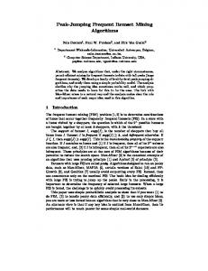
The FP-Growth tree will be constructed as below figure 1.
1.Scan the transaction database DB once. Collect the set of frequent items F and their supports. Sort F in support descending order as L, the list of frequent items. 2.Create the root of an FP-tree, T, and label it as “root”. For each transaction Trans in DB do the following: 1.Select and sort the frequent items in Trans according to the order of L. Let the sorted frequent item list in Trans be [p | P], where p is the first element and P is the remaining list. Call insert_tree([p | P], T). 2.The function insert_tree([p | P], T) is performed as follows. If T has a child N such that N.item-name = p.item-name, then increment N’s count by 1; else create a new node N, and let its count be 1, its parent link be linked to T, and its node-link be linked to the nodes with the same item-name via the node-link structure. If P is nonempty, call insert_tree(P, N) recursively.
Figure 1: An example of a FP-tree.
3.4 Eclat 3.2. Broglet’s FP-Growth Broglet implemented an efficient FP-Growth[1] algorithm using C Language. The FP-growth in his implementation preprocesses the transaction database according to [1] is as follows: 1.In an initial scan the frequencies of the items (support of single element item sets) are determined. 2. All infrequent items, that is, all items that appear in fewer transactions than a user-specified minimum number are discarded from the transactions, since, obviously, they can never be part of a frequent item set. 3. The items in each transaction are sorted, so that they are in descending order with respect to their frequency in the database.
3.3. Goethals FP-Growth Goethal also implemented the FP-Growth algorithm. This implementation is based on the Fp-growth algorithm [5]. Consider a transaction database and a minimal support threshold of 2. First, the supports of all items is computed, all infrequent items are removed from the database and all transactions are reordered according to the support descending order resulting in the example transaction database in Table 1. The FP-tree for this database is shown in Figure 1.
Eclat [11, 8, 3] algorithm is basically a depth-first search algorithm using set intersection. It uses a vertical database layout i.e. instead of explicitly listing all transactions; each item is stored together with its cover (also called tidlist) and uses the intersection based approach to compute the support of an itemset. In this way, the support of an itemset X can be easily computed by simply intersecting the covers of any two subsets Y, Z ⊆ X, such that Y U Z = X. It states that, when the database is stored in the vertical layout, the support of a set can be counted much easier by simply intersecting the covers of two of its subsets that together give the set itself.
The Eclat algorithm is as given below. Input: D, σ, i ⊆ I Output: F[I](D, σ) 1: F[I] :={} 2: for all I Є I occurring in D do 3: F[I] := F[I] ∪ {I ∪ {i}} 4: // Create Di
Table 1: An example preprocessed transaction database.
5: Di: = {} 6: for all j Є I occurring in D such that j>I do
Tid
X
7: C := cover({i}) ∩ cover({j}) 8: if |C| >= σ then 87
International Journal of Computer Applications (0975 - 8887) Volume 1 – No. 15
9: Di: = Di ∪ {(j, C)} 10: end if 11: end for 12: //Depth-first recursion 13: Compute F[I ∪ {i}](Di, σ) 14: F[I] := F[I] ∪ F[I ∪ {i}] 15: end for In this algorithm each frequent item is added in the output set. After that, for every such frequent item i, the i-projected database Di is created. This is done by first finding every item j that frequently occurs together with i. The support of this set {i, j} is computed by intersecting the covers of both items. If {i, j} is frequent, then j is inserted into Di together with its cover. The reordering is performed at every recursion step of the algorithm between line 10 and line 11. Then the algorithm is called recursively to find all frequent itemsets in the new database Di. It essentially generates the candidate itemsets using only the join step from Apriori. Again all the items in the database is reordered in ascending order of support to reduce the number of candidate itemsets that is generated, and hence, reduce the number of intersections that need to be computed and the total size of the covers of all generated itemsets. Since the algorithm doesn’t fully exploit the monotonicity property, but generates a candidate itemset based on only two of its subsets, the number of candidate itemsets that are generated is much larger as compared to a breadth-first approach such as Apriori. As a comparison, Eclat essentially generates candidate itemsets using only the join step from Apriori [6], since the itemsets necessary for the prune step are not available. A technique that is regularly used is to reorder the items in support ascending order to reduce the number of candidate itemsets that is generated. In Eclat, such reordering can be performed at every recursion step in the algorithm. Also that at a certain depth d, the covers of at most all k-itemsets with the same k − 1-prefix are stored in main memory, with k < d. Because of the item reordering, this number is kept small.
3.5 SaM Algorithm The SaM (Split and Merge) algorithm established by [10] is a simplification of the already fairly simple RElim (Recursive Elimination) algorithm. While RElim represents a (conditional) database by storing one transaction list for each item (partially vertical representation), the split and merge algorithm employs only a single transaction list (purely horizontal representation), stored as an array.
1. The transaction database is taken in its original form. 2. The frequencies of individual items are determined from this input in order to be able to discard infrequent items immediately. 3. The (frequent) items in each transaction are sorted according to their frequency in the transaction database, since it is well known that processing the items in the order of increasing frequency usually leads to the shortest execution times. 4. The transactions are sorted lexicographically into descending order, with item comparisons again being decided by the item frequencies; here the item with the higher frequency precedes the item with the lower frequency. 5. The data structure on which SaM operates is built by combining equal transactions and setting up an array, in which each element consists of two fields: An occurrence counter and a pointer to the sorted transaction (array of contained items). This data structure is then processed recursively to find the frequent item sets. The basic operations of the recursive processing are based on depth-first/divide-andconquer scheme. In the split step the given array is split with respect to the leading item of the first transaction. All array elements referring to transactions starting with this item are transferred to a new array. The new array created in the split step and the rest of the original arrays are combined with a procedure that is almost identical to one phase of the well-known merge sort algorithm.The main reason for the merge operation in SaM is to keep the list sorted, so that: 1.All transactions with the same leading item are grouped together and 2.Equal transactions (or transaction suffixes) can be combined, thus reducing the number of objects to process.
Figure 2: Transaction database (left), item frequencies (middle), and reduced transaction database with items in transactions sorted accordingly with respect to their frequency (right). Each transaction is represented as a simple array of item identifiers (which are integer numbers). The transaction list is prepared which are stored in a simple array, each element of which contains a support counter and a pointer to the head of the list. The list elements themselves consist only of a successor pointer and a pointer to the transaction. The transactions are
inserted one by one into this structure by simply using their leading item as an index.
This array is processed with a simple split and merge scheme, which computes a conditional database, processes this conditional database recursively, and finally eliminates the split item from the original (conditional) database. SaM preprocesses a given transaction following the steps below: 88
International Journal of Computer Applications (0975 - 8887) Volume 1 – No. 15 taken and the number of Itemsets Generated for different data sets. For this comparison also same data sets were selected as for the above experiment with 30% to 70% of minimum support threshold. The table 3 below shows the execution time for all the algorithms with different support threshold for adult data set. The time of execution is decreased with the increase support threshold.
Table 3: Adult data set execution time. Total Time in Seconds Support
Figure 3: Procedure of the recursive elimination with the modification of the transaction lists (left) as well as the transaction lists for the recursion (right).
4. Data Set Requirements For the experiment we have used datasets of different application. These datasets was obtained from the UCI repository of machine learning databases [7]. The Table 2 below portraits the characteristics of the datasets selected for the experiment. Table 2: Details of Datasets used in the comparison
File name
Divisi ons
Dist./ Rand.
Recor ds
BROGLET FP-Growth
Eclat
Relim
SaM
30
0.56
0.54
0.49
0.47
40
0.5
0.49
0.44
0.44
50
0.49
0.45
0.42
0.41
60
0.48
0.44
0.4
0.4
70
0.42
0.4
0.39
0.37
Figure 4 shows that the execution time for the FP-growth algorithm decreases with the increase in support threshold form 30% to 70% for adult dataset. We observed that FP-growth and Eclat takes more time as that compared to RElim and SaM.
Comparison of FIM Algorithms
I/P Columns
0.6 BROGLET FPGrowth
adult.D97.
5
Yes
48842
15
N48842.C2.n um
Time in Sec.
0.55
BROGLET Eclat
0.5
BROGLET Relim
0.45
BROGLET SaM
0.4 0.35 30
40
50
60
70
Support
Census
0
No
48842
14 Figure 4: Execution Time for adult data set.
letRecog.D1 06. N20000.C26. num
5
Mushroom.
5
Yes
20000
17 The table 4 shows the execution time for all the algorithms with different support threshold for census data set. The time of execution is decreased with the increase support threshold.
Yes
8124
23
D90.N8124. C2.num
5.Performance Comparisons We have conducted a detailed study to assess the performance of FP-Growth with respect to the other FIM algorithms. The performance metrics in the experiments is the total execution time 89
International Journal of Computer Applications (0975 - 8887) Volume 1 – No. 15 Figure 6 shows that the execution time of the FP-growth algorithm is near by the execution time of Eclat and RElim with the decrease in support threshold for Letter Recognition data set. It is also analyzed that the execution time for other SaM algorithm is less as compared to other FIM algorithms.
Table 4: Census data set execution time.
Total Time in Seconds BROGLET
Support FPGrowth
Eclat
30
1.21
0.76
0.74
0.74
40
1.16
0.75
0.72
0.71
Relim
SaM Comparison of FIM Algorithms
0.86
0.72
0.7
0.69
60
0.73
0.69
0.67
0.67
70
0.68
0.65
0.65
0.2 Time in Sec.
50
0.22
0.18
FP-Growth Eclat
0.16
Relim
0.14
SaM
0.12
0.64
0.1 30
40
50
60
70
Support
Figure 5 shows that the execution time for the FP-growth algorithm is high with the small support threshold and it decreases with the decrease in support using census data set. It is also analyzed that the execution time for other FIM algorithms is less as compared to FP-growth algorithm. Comparison of FIM Algorithms 1.3
The table 7 below shows the execution time for all the algorithms with different support threshold for mushroom data set. The time of execution is decreased with the increase support threshold.
Table 7: Mashroom data set execution time.
1.2 Time in Sec.
Figure 6: Execution Time for Letter Recognition data set.
1.1
FP-Growth
1
Eclat
Total Time in Seconds
Relim
0.9
SaM
0.8
BROGLET
Support
0.7
FPGrowth
Eclat
Relim
30
0.13
0.11
0.11
0.11
Figure 5: Execution Time for census data set.
40
0.11
0.11
0.09
0.1
The table 5 below show the execution time for all the algorithms with different support threshold for Letter Recognition data set. The time of execution is decreased with the increase support threshold.
50
0.09
0.09
0.09
0.08
60
0.08
0.09
0.08
0.07
70
0.08
0.08
0.07
0.06
0.6 30
40
50
60
70
Support
Table 5: Letter Recognition data set execution time
SaM
Figure 7 shows that the execution time of the all FIM algorithm is nearby but it can also be analyzed that the execution time of SaM is comparatively less for higher support threshold.
Total Time in Seconds BROGLET
Support
Comparison of FIM Algorithms
FPGrowth
Eclat
30
0.21
0.21
0.2
0.19
40
0.2
0.21
0.19
0.18
Relim
SaM
0.14 0.13
50
0.18
0.2
0.19
0.17
60
0.17
0.19
0.18
0.16
70
0.15
0.17
0.16
0.14
Time in Sec.
0.12 0.11
FP-Growth
0.1
Eclat
0.09
Relim
0.08
SaM
0.07 0.06 0.05 30
40
50
60
70
Support
Figure 7: Execution Time for Mushroom data set. 90
International Journal of Computer Applications (0975 - 8887) Volume 1 – No. 15
6.Findings and Analysis The first interesting behavior can be observed in the Experiment 1 for the adult, census and letter recognition data set. Indeed, Broglet’s FP performs better for adult and letter data set, as it takes much less time to generate frequent itemsets in comparison of Goethal’s FP. Whereas for letter recognition data set Goethal’s FP takes much less time of execution then the other, but it can also be studied that it generates constant number of frequent itemsets even with the increase in the minimum support threshold. Another remarkable result is that the frequent itemsets generated by Goethal’s is enormous then that generated by the Broglet’s FP of which numerous itemsets may not be useful from the point of mining purpose. Future no. of transaction of adult and census data set are same, even then Goethal’s FP behave inappropriate for census data set.By these consequences we consider Broglet’s FP to be better performer than that of Goethal’s FP and accordingly we performed the second experiment to compare the Broglet’s FP with the classical frequent itemset mining algorithms (like Apriori and Eclat) along with the newly implemented algorithms (RElim and SaM). In the later experiment it can be observed that for adult and census data set FP-Growth takes more time than that of other FIM algorithms. Along that RElim performs in close proximity to that of SaM. For letter recognition and mushroom dataset all the FIM algorithms performs close to each other. Nevertheless, SaM can be considered as an improved performer from the overall dataset analysis.
7.CONCLUSION A comparison framework has developed to allow the flexible comparison of existing and new frequent itemset mining algorithms that conform to the defined algorithm interface. Using this framework this paper presented the comparative performance study of three iterative algorithms for FIM algorithms with FPGrowth algorithms. In this work, an in-depth analysis of few algorithms is done which made a significant contribution to the search of improving the efficiency of frequent itemset mining. By comparing them to classical frequent item set mining algorithms like FP-growth and Eclat the strength and weaknesses of these algorithms were analyzed. The developed framework can be used for comparing the other algorithms, which does not use candidate set generation to discover frequent patterns. And can also lead to several ideas for optimizations, which could improve the performance of other algorithms.
8. REFERENCE [1]
C. Borgelt. An Implementation of the FP- growth Algorithm. Proc. Workshop Open Software for Data Mining (OSDM’05 at KDD’05, Chicago,IL),1–5.ACMPress, New York, NY, USA 2005.
[2]
C.Borgelt. Keeping Things Simple: Finding Frequent Item Sets by Recursive Elimination. Proc. Workshop Open Software for Data Mining (OSDM’05 at KDD’05, Chicago, IL), 66– 70. ACM Press, New York, NY, USA 2005.
[3]
C.Borgelt. Efficient Implementations of Apriori and Eclat. Proc. 1st IEEE ICDM Workshop on Frequent Item Set Mining Implementations (FIMI 2003, Melbourne, FL). CEUR Workshop Proceedings 90, Aachen, Germany 2003.
[4]
J. Han, J. Pei, Y. Yin, and R. Mao. Mining frequent patterns without candidate generation: A frequent-pattern tree approach. Data Mining and Knowledge Discovery, 2003.
[5]
J. Han, H. Pei, and Y. Yin. Mining Frequent Patterns without Candidate Generation. In: Proc. Conf. on the Management of Data (SIGMOD’00, Dallas, TX). ACM Press, New York, NY, USA 2000.
[6 ] R. Agrawal, H. Mannila, R. Srikant, H. Toivonen, and A.I. Verkamo. Fast discovery of association rules. In U.M. Fayyad, G. Piatetsky-Shapiro, P. Smyth, and R. Uthurusamy, editors, Advances in Knowledge Discovery and Data Mining, pages 307–328. MIT Press, 1996. [7 ] C.L. Blake and C.J. Merz. UCI Repository of Machine Learning Databases. Dept. of Information and Computer Science, University of California at Irvine, CA, USA1998 http://www.ics.uci.edu/˜mlearn/MLRepository.html- 1998. [8]
[9]
M. Zaki, S. Parthasarathy, M. Ogihara, and W. Li. NewAlgorithms for Fast Discovery of Association Rules. Proc. 3rd Int. Conf. on Knowledge Discovery and Data Mining (KDD’97), 283–296. AAAI Press, Menlo Park, CA, USA 1997. R. Agrawal, T. Imielienski, and A. Swami. Mining Association Rules between Sets of Items in Large Databases. Proc. Conf. on Management of Data, 207–216. ACM Press, New York, NY, USA 1993.
[10] C. Borgelt. SaM: Simple Algorithms for Frequent Item Set Mining. IFSA/EUSFLAT 2009 conference- 2009. [11] J. Han, and M. Kamber, 2000. Data Mining Concepts and Techniques. Morgan Kanufmann.
91