By Kai Schneiderâ , Marie Fargeâ¡, Giulio Pellegrino¶ AND Michael Rogers. Coherent Vortex Simulation (CVS) filtering has been applied to DNS data of forced.
319
Center for Turbulence Research Proceedings of the Summer Program 2000
CVS filtering of 3D turbulent mixing layers using orthogonal wavelets By Kai Schneider†, Marie Farge‡, Giulio Pellegrino¶
AND
Michael Rogersk
Coherent Vortex Simulation (CVS) filtering has been applied to DNS data of forced and unforced time-developing turbulent mixing layers. CVS filtering splits the turbulent flow into two orthogonal parts, one corresponding to coherent vortices and the other to incoherent background flow. We have shown that the coherent vortices can be represented by few wavelet modes and that these modes are sufficient to reproduce the vorticity probability distribution function (PDF) and the energy spectrum over the entire inertial range. The remaining incoherent background flow is homogeneous, has small amplitude, and is uncorrelated. These results are compared with those obtained for the same compression rate using large eddy simulation (LES) filtering. In contrast to the incoherent background flow of CVS filtering, the LES subgrid scales have a much larger amplitude and are correlated, which makes their statistical modeling more difficult.
1. Introduction In the turbulent regime the solutions of Navier-Stokes equations exhibit coherent vortices whose nonlinear interactions are responsible for the flow evolution. Since these coherent vortices are well localized and excited on a wide range of scales, we have proposed to use the wavelet representation of the vorticity field to extract them (Farge, Schneider & Kevlahan (1999)). Orthogonal wavelet bases are well suited for this because they are made of self-similar functions well localized in both physical and spectral spaces (Farge (1992), Daubechies (1992)). In (Farge, Schneider & Kevlahan (1999)) we have introduced a new method, called Coherent Vortex Simulation (CVS), to compute turbulent flows. It is based on the wavelet filtered Navier-Stokes equations and their solution in an adaptive wavelet basis which is dynamically adapted during the flow evolution (Schneider & Farge (2000)). Here we first present the vector valued wavelet algorithm used to extract coherent vortices out of turbulent flows. Then we employ this algorithm to analyze DNS computations of two time-developing three-dimensional turbulent mixing layers (Rogers & Moser (1994)). The results are compared with those obtained for the same compression using an ideal low-pass filter, as used for LES computation. Finally, we draw some conclusions for developing CVS computations for three-dimensional turbulent flows.
2. Wavelet method for coherent vortex extraction In (Farge, Schneider & Kevlahan (1999), Farge, Pellegrino & Schneider (2000)) we have proposed a wavelet-based method to extract coherent vortices out of 2D and 3D turbulent † ‡ ¶ k
CMI, Universit´e de Provence, Marseille, France LMD-CNRS, Ecole Normale Sup´erieure, Paris, France ICT, Universit¨ at Karlsruhe (TH), Germany NASA Ames Research Center, Moffett Field, CA
320
K. Schneider, M. Farge, G. Pellegrino & M. Rogers
flows. The algorithm for the 3D case is described below. We consider the vorticity field ~ , computed at resolution N = 23J , N being the number of grid points ~ω (~x) = ∇ × V and J the number of octaves. Each component is developed into an orthogonal wavelet series from the largest scale lmax = 20 to the smallest scale lmin = 2J−1 using a 3D multi-resolution analysis (MRA) (Daubechies (1992), Farge (1992)): ω(~x) = ω ¯ 0,0,0 φ0,0,0 (~x)
+
j j j n J−1 −1 2X −1 2X −1 2X −1 X 2X
µ µ ω ˜ j,i ψj,i (~x) x ,iy ,iz x ,iy ,iz
, (2.1)
j=0 ix =0 iy =0 iz =0 µ=1
with
φj,ix ,iy i,iz (~x) = φj,ix (x) φj,iy (y) φj,iz (z), and ψj,ix (x) φj,iy (y) φj,iz (z) φj,ix (x) ψj,iy (y) φj,iz (z) φj,ix (x) φj,iy (y) ψj,iz (z) µ ψj,ix (x) φj,iy (y) ψj,iz (z) ψj,i (~ x ) = x ,iy ,iz ψj,ix (x) ψj,iy (y) φj,iz (z) φj,ix (x) ψj,iy (y) ψj,iz (z) ψj,ix (x) ψj,iy (y) ψj,iz (z)
; ; ; ; ; ; ;
µ=1 µ=2 µ=3 µ=4 µ=5 µ=6 µ=7
, , , , , , ,
(2.2)
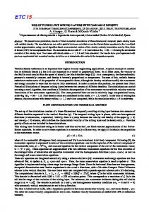
where φj,i and ψj,i are the one-dimensional scaling function and the corresponding wavelet, respectively. Due to orthogonality, the scaling coefficients are given by ω ¯ 0,0,0 = µ µ hω , φ0,0,0 i and the wavelet coefficients are given by ω ˜ j,i = hω , ψ i, where j,ix ,iy ,iz x ,iy ,iz 2 h·, ·i denotes the L -inner product. We then split the vorticity field into ~ωC (~x) and ~ωI (~x) by applying a nonlinear thresholding to the wavelet coefficients. The threshold is defined as � = (4/3Z log N )1/2 , and it only depends on the total enstrophy Z and on the number of grid points N without any adjustable parameters. The choice of this threshold is based on theorems (Donoho (1993), Donoho & Johnstone (1994)) proving optimality of the wavelet representation to denoise signals in the presence of Gaussian white noise since this wavelet-based estimator minimizes the maximal L2 -errorfor functions with inhomogeneous regularity. The coherent vorticity field ~ωC is reconstructed from the wavelet coefficients whose modulus is larger than � and the incoherent vorticity field ~ωI from the wavelet coefficients whose modulus is smaller or equal to �. The two fields thus obtained, ~ωC and ~ωI , are orthogonal, which ensures a separation of the total enstrophy into Z = ZC + ZI because the ~ = ∇ × (∇−2 ω ~) interaction term h~ωC , ~ωI i vanishes. We then use Biot-Savart’s relation V ~ ~ to reconstruct the coherent velocity VC and the incoherent velocity VI for the coherent and incoherent vortices, respectively. In the present paper we apply the above algorithm to two high resolution direct numerical simulations (DNS) of 3D turbulent flows with a Taylor microscale Reynolds number of about Rλ = 150. The first computation is a forced mixing layer computed at resolution 384 × 120 × 128 and evolved for 40 eddy turnover times (Rogers & Moser (1994)). The vorticity field is interpolated onto a physical space grid that is either coarsened to N = 643 for flow visualization (Fig. 1, Fig. 2), or refined to N = 512 × 256 × 128 in order to compute the energy spectra and vorticity PDFs using the full resolution compatible with the dyadic wavelet representation (Fig. 3). The second computation is an unforced mixing layer computed at resolution 512 × 180 × 192 and evolved for 60 eddy turnover times (Rogers & Moser (1994)). Again the vorticity has been interpolated onto different physical space grids for flow visualization (N = 643 for Fig. 5, Fig. 6, and Fig. 8), and statistical analysis (N = 512 × 256 × 128 for Fig. 7).
CVS filtering of 3D turbulent mixing layers
321
0.00
Y
0.00 0.00 3 2
Z
X
100% N 100% Z
1 0
|ω|
Figure 1. Total vorticity of the forced 3D mixing layer at resolution N = 643 .
3. Application to the forced mixing layer Figure 1 shows the modulus of vorticity for the total flow in the forced case (at low resolution N = 643 ). We observe well pronounced longitudinal vortex tubes, called ribs, which result from a 3D instability and are wrapped onto four transverse rollers that are produced by the 2D Kelvin-Helmholtz instability. The coherent vorticity (see Fig. 2 top), which is contained in 5.7% (at low resolution N = 643 ) or 3% (at high resolution N = 512 × 256 × 128) of the total number N of wavelet coefficients, captures most of the turbulent kinetic energy and enstrophy, even at high wavenumbers. Moreover, the PDF of the coherent vorticity is similar to that of the total flow (see Fig. 3 bottom left). The incoherent vorticity (see Fig. 2 bottom), which is represented by 94.3% (at low resolution N = 643 ) or 97% (at high resolution N = 512×256×128) of the total number N of wavelet coefficients, contains little of the turbulent kinetic energy and enstrophy. It is nearly homogeneous with a very low amplitude and contains no structure. The PDF of the incoherent vorticity (Fig. 3 bottom left) follows an exponential law with a much reduced variance compared to the PDF of the total flow. The similarity between the 1D energy spectra (Fig. 3 top left) in the streamwise direction for the coherent part of the flow and for the total flow indicates that the energetic turbulent motions are well captured by the filtering. In contrast, the incoherent part contains very little energy and is well uncorrelated with flat energy spectrum. In Fig. 4 we display vertical profiles of the three vorticity components ωx , ωy , ωz averaged in the streamwise and spanwise directions. Examination of the the spanwise component ωz (Fig. 4, bottom) shows that the coherent vorticity exactly follows the total vorticity, while the incoherent vorticity oscillates weakly around zero with amplitudes less than 4% of the minimal value ω ¯ z,min . The vertical component ωy (Fig. 4, middle) of the total flow vanishes since the flow is homogeneous in the streamwise and spanwise directions. The coherent and incoherent components oscillate around zero with amplitudes of about 1% of ω ¯ z,min . The streamwise component ωx profiles (Fig. 4, top) are similar to the spanwise ones in that the coherent component follows the total one, while
322
K. Schneider, M. Farge, G. Pellegrino & M. Rogers
0.00
Y
0.00 0.00 3 2
Z
X
5.7% N 64.3% Z
1 0
|ω|
0.00
Y
0.00 0.00 3 2
Z
X
94.3% N 37.5% Z
1 0
|ω|
Figure 2. Forced mixing layer. Top: Coherent vorticity. Bottom: Incoherent vorticity.
the incoherent vorticity oscillates weakly around zero with amplitudes less than 4% of the minimal value ω ¯ z,min .
4. Application to the unforced mixing layer Figure 5 shows the modulus of vorticity for the total flow for the unforced mixing layer at resolution N = 643 . In contrast to the forced mixing layer (Fig. 1), we observe much less pronounced longitudinal vortex tubes and transverse rollers, with little, if any, large-scale structures. The coherent vorticity (Fig. 6 top), which is contained in 8% (at low resolution N = 643 ) or 3% (at high resolution N = 512 × 256 × 128) of the total number N of wavelet
CVS filtering of 3D turbulent mixing layers
323
1D energy spectra E(k_x) -1
-1
10
10
E_v, total
-2
10
E_v, incoherent
-3
10
-3
10
-4
-4
10
-5
10
-6
10
-7
10
10
-5
10
-6
10
E_v, low
E_v, high
-7
10
-8
-8
10
E_v, total
-2
10
E_v, coherent
10 -2
-1
10
0
10
10
1
-2
2
10
-1
10
10
0
10
1
10
2
10
10
k_x
k_x
Vorticity PDF p(ω) 1
10
0
p(w_y), total p(w_y), coherent p(w_y), incoherent
10
-1
10
-2
10
-3
10
-4
10
-5
10
-6
10
-7
10
-10
-5
0
w
5
10
10
1
10
0
10
-1
10
-2
10
-3
10
-4
10
-5
10
-6
10
-7
p(w_y), total p(w_y), low p(w_y), high
-10
-5
0
5
10
w
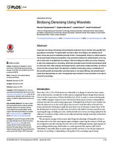
Figure 3. Comparison of CVS (left) with LES (right) filtering for the forced mixing layer at resolution N = 512 × 256 × 128. Energy spectra (top) and PDF of vorticity (bottom) of total, coherent (3% N) and incoherent (97% N) flow using CVS filtering and of low wavenumber and high wavenumber components using LES filtering.
coefficients, shows small-scale organized structures, while the incoherent vorticity (Fig. 6 bottom), which represents 92% (at low resolution N = 643 ) or 97% (at high resolution N = 512 × 256 × 128) of the total number N of wavelet coefficients, is homogeneous, structureless, and has a much weaker amplitude. This is also confirmed by the vorticity PDF (Fig. 7 bottom left), where the coherent vorticity presents the same non-Gaussian distribution as the total vorticity. In contrast, the incoherent vorticity follows an exponential law with a much reduced variance compared to the total vorticity. Moreover, we have verified, as for the forced case, that the coherent flow has the same spectral distribution as the total flow for all but the highest dissipative wavenumbers (Fig. 7 top left), while the incoherent flow is uncorrelated and exhibits a flat energy spectrum.
324
K. Schneider, M. Farge, G. Pellegrino & M. Rogers
0.03 0.02
ωx
0.01 0 -0.01 -0.02 -0.03
0
10
20
30
40
50
60
0
10
20
30
40
50
60
0
10
20
30
40
50
60
0.004 0.003 0.002
ωy
0.001 0 -0.001 -0.002 -0.003 -0.004 0.05 0
ωz
-0.05 -0.1 -0.15 -0.2 -0.25
y Figure 4. Averaged cuts of ωx , ωy , ωz for total, coherent and incoherent vorticity for the , total; , coherent; , incoherent. forced mixing layer. Symbols:
CVS filtering of 3D turbulent mixing layers
325
0.00
Y
0.00 0.00
Z
X
100% N 100% Z
Figure 5. Total vorticity of the unforced 3D mixing layer at resolution N = 643 .
5. Comparison between CVS and LES filtering We now consider the results obtained with the LES filtering applied to the two time developing mixing layers we have studied. We choose the simplest LES filter and use a low-pass Fourier filter with a cut-off at the wavenumber k = 25, which therefore retains 9% of the N = 512 × 256 × 128 Fourier modes. The discarded Fourier modes correspond to the subgrid scales. This comparison is actually quite unfair for the CVS filtering since it retains even less, namely 3% of the N wavelet modes. The LES filtering keeps only the scales larger than the cutoff wavenumber (Fig. 3 and 7 top, right), and hence the coherent vortices are smoothed. As a result, the extrema of vorticity are strongly reduced (see PDF on Fig. 3 and 7 bottom, right). In contrast, the CVS filtering retains the organized features, whatever their scales, and in this case the shape of the vorticity PDF is fully preserved even for large values of vorticity (Fig. 3 and 7 bottom, left). If we now consider the results obtained with the LES filtering applied to the unforced mixing layer for the same compression rate, we observe that both low and high wavenumber components (Fig. 8) present localized structures and that the vorticity PDF for both components (Fig. 7 right) has about the same variation. In fact the high wavenumber modes, which ought to be modeled in LES to avoid numerical divergence, have a more non-Gaussian distribution than the low wavenumber modes which are resolved by LES; therefore, the turbulence modeling cannot be based on the assumption of a Gaussian behavior for the discarded high wavenumber modes. Concerning turbulence parameterization, i.e. the statistical modeling of the effect of the discarded modes on the retained modes, we can draw the following conclusions: • The CVS filtering disentangle the organized from random components of turbulent flows. • The LES filtering does not produce subgrid-scale modes that are uncorrelated, and there are, therefore, many organized structures present in the subgrid-scale flow that can interact nonlinearly and transfer energy back to larger scales (backscatter). • The incoherent modes discarded by CVS have very weak amplitude, are almost ho-
326
K. Schneider, M. Farge, G. Pellegrino & M. Rogers
0.00
Y
0.00 0.00
Z
X
8% N 62% Z
0.00
Y
0.00 0.00
Z
X
100% N 100% Z
Figure 6. Unforced mixing layer. Top: Coherent vorticity. Bottom: Incoherent vorticity.
mogeneous in space, and are well decorrelated, which should avoid the transfer of energy from the incoherent modes to the coherent modes and, therefore, controls backscattering. • The variability of the total field is not retained by the LES filtering and, as a consequence, the discarded high-wavenumber modes contain much more vorticity than the incoherent modes discarded by the CVS filtering. • For LES, if we do not model the effect of the subgrid scale modes on the resolved modes, the energy accumulates at the cutoff and the computation diverges. • For CVS, if we do not model the effect of the discarded incoherent modes on the resolved coherent modes, there is no risk of divergence since energy can be transferred in both directions all along the fully resolved inertial range – the only consequence of no turbulence model may be some extra dissipation. We conjecture that the derivation of a turbulence model is easier with CVS filter-
CVS filtering of 3D turbulent mixing layers
327
1D energy spectra E(k_x) -2
-2
10
10
E_v, total E_v, coherent E_v, incoherent
-3
10
E_v, total -3
10 -4
10
-4
10 -5
10
E_v, low
-5
10
E_v, high
-6
10
-6
10
-7
10
-2
-1
10
0
10
1
10
-2
-1
10
2
10
10
0
10
1
10
2
10
10
k_x
k_x
Vorticity PDF p(ω) 1
1
10
10
p(w_y), total 0 10 p(w_y), coherent p(w_y), incoherent
0
10
10
10
-2
-2
10
-3
10
-4
10
-5
10
-6
10
10
-3
10
-4
10
-5
10
-6
10
-7
-7
10
-12
p(w_y), total p(w_y), low p(w_y), high
-1
-1
-8
-4
0
ω
4
8
10 -12 12
-8
-4
0
4
8
12
ω
Figure 7. Comparison of CVS (left) with LES (right) filtering for the unforced 3D mixing layer, at resolution N = 512 × 256 × 128. Energy spectra (top) and PDF of vorticity (bottom) of total, coherent (3% N) and incoherent (97% N) flow using CVS filtering and of low wavenumber and high wavenumber components using LES filtering.
ing than with LES filtering because the discarded modes in this case are statistically well behaved, homogeneous, uncorrelated, and have an exponential PDF with a small variability.
6. Divergence problem Due to the fact that the CVS filtering is nonlinear and the vector valued wavelet ~λ 6= 0, the CVS filtering does not yield coherent basis is not divergence-free, i.e. ∇ · ψ and incoherent vorticity that is completely divergence-free. For the flow examined here, however, the divergent contribution of the vorticity field was less than 3% of the total enstrophy. The same problem is also encountered for vortex methods applied to 3D turbulent flows (Winckelmans (1995)). However, the corresponding velocity fields are
328
K. Schneider, M. Farge, G. Pellegrino & M. Rogers
0.00
Y
0.00 0.00
Z
X
8% N 48% Z
0.00
Y
0.00 0.00
Z
X
92% N 52% Z
Figure 8. Unforced case. Top: Low wavenumber vorticity of the turbulent mixing layer reconstructed from 8% of the wavelet coefficients and containing 48% of the total enstrophy. Bottom: High wavenumber vorticity reconstructed from 92% of the Fourier coefficients and containing 52% of the total enstrophy.
divergence-free since they have been reconstructed using the Biot-Savart kernel. There are several possible ways to insure that the coherent vorticity remains divergence-free: • use divergence-free orthogonal wavelets (Lemari´e (1992)), • decompose ω into ω = ωdiv=0 + ∇φ. Then φ can be calculated by taking the divergence which leads to a Poisson equation ∇2 φ = ∇ · ω. • apply the previous decomposition, not to the solution, but to the wavelet basis itself, which can be done as a precalculation since the wavelet decomposition is a linear transformation.
CVS filtering of 3D turbulent mixing layers
329
7. Conclusion and perspectives The CVS method is based on the projection of the vorticity field on an orthogonal wavelet basis and the decomposition of the vorticity field into two orthogonal components, using a nonlinear thresholding of the wavelet coefficients. The coherent vorticity field is reconstructed from the few wavelet coefficients larger than a given threshold, which depends only on the resolution and on the total enstrophy, while the incoherent vorticity is reconstructed from the many remaining weak wavelet coefficients. The coherent and incoherent velocity fields are then derived from the coherent and incoherent vorticity fields using Biot-Savart’s equation. In this paper we have applied this method to two 3D time developing mixing layers, forced and unforced, at resolution N = 512×256×128. We have shown that the coherent flow corresponds to only 3%N wavelet modes, presents the same non-Gaussian PDF of vorticity, and retains most of the energy and enstrophy, with the same spectral distribution, as the total flow. Moreover, the remaining incoherent flow is structureless, exhibits a much narrower PDF of vorticity with an exponential distribution, and presents an energy equipartition spectrum. This suggests the possibility of parameterizing the effect of the incoherent flow on the coherent flow using a low-order statistical model. The advantage of the CVS filtering in comparison to the LES filtering was also demonstrated. The small scale flow, which is discarded in LES and replaced by a subgrid scale model, exhibits many coherent structures, has a much wider PDF of vorticity, and does not present an energy equipartition spectrum. The success of the CVS filtering procedure suggests the possibility of extending the CVS method to solve the 3D Navier-Stokes equations directly in an adaptive wavelet basis. In (Schneider & Farge (2000)) we have shown that the CVS computation of a 2D mixing layer gives the same results as those from a standard DNS. The dynamical adaption of the grid in physical space allows the important coherent part of the flow to be evolved with a reduced number of active degrees of freedom. Thus the CVS computation combines a Eulerian representation of the flow with a Lagrangian adaption strategy for the active degrees of freedom, which are remapped at each time step using the CVS filtering.
Acknowledgments M. F. and K. S. thankfully acknowledge financial support from the Center for Turbulence Research, Stanford University.
REFERENCES
Daubechies, I. 1992 it Ten Lectures on wavelets. SIAM, Philadelphia. Donoho, D. 1993 Unconditional bases are optimal bases for data compression and statistical estimation. Appl. Comput. Harmon. Anal. 1, 100. Donoho, D. & Johnstone, I. 1994 Ideal spatial adaption via wavelet shrinkage. Biometrica. 81, 425-455. Farge, M. 1992 Wavelet Transforms and their Applications to Turbulence. Ann. Rev. of Fluid Mech. 24, 395-457. Farge, M., Schneider, K., & Kevlahan, N. 1999 Non-Gaussianity and Coherent Vortex Simulation for two-dimensional turbulence using an adaptive orthonormal wavelet basis. Phys. Fluids 11(8), 2187-2201.
330
K. Schneider, M. Farge, G. Pellegrino & M. Rogers
Farge, M. & Schneider, K. 2000 Coherent Vortex Simulation (CVS), a semideterministic turbulence model using wavelets. Flow, Turb. Combust., submitted. Farge, M., Pellegrino, G. & Schneider, K. 2000 Coherent vortex extraction in 3D turbulent flows using orthogonal wavelets. Phys. Rev. Lett., submitted. Lemari´ e P. G. 1992, Analyses multir´esolutions non orthogonales, commutation entre projecteurs de d´erivation et ondelettes a` divergence nulle. Revista Mat. Iberoamericana. 8, 221-236. Rogers, M. & Moser, R. 1994 Direct simulation of a self-similar turbulent mixing layer. Phys. Fluids. 6(2), 903-923. Schneider, K. & Farge, M. 1997 Wavelet forcing for numerical simulation of twodimensional turbulence. C. R. Acad. Sci. Paris, S´erie II b. 325, 263-270. Schneider, K. & Farge, M. 1998 Wavelet approach for modelling and computing turbulence. Lecture Series 1998-05 Advances in turbulence modelling. Von Karman Institute for Fluid Dynamics, Bruxelles, 132 pages. Schneider, K. & Farge, M. 2000 Numerical simulation of temporally growing mixing layer in an adaptive wavelet basis. C. R. Acad. Sci. Paris S´erie II b. 328, 263-269. Winckelmans, G. S. 1995 Some progress in large-eddy simulation using the 3D vortex particle method. Annual Research Briefs, Center for Turbulence Research, NASA Ames/Stanford Univ. 391-415.