Transactions of the Institute of Measurement and Control 23,2 (2001) pp. 69â82. D-Type learning control for nonlinear time-varying systems with unknown initial ...
Transactions of the Institute of Measurement and Control 23,2 (2001) pp. 69–82
D-Type learning control for nonlinear time-varying systems with unknown initial states and inputs X.G. Yan,1 I.M. Chen1 and J. Lam2 1
School of Mechanical and Production Engineering, Nanyang Technological University, Nanyang Avenue, Singapore 639798 2 Department of Mechanical Engineering, University of Hong Kong, Pokfulam Road, Hong Kong
In this paper, D-type iterative learning control schemes, which guarantee that the desired output is tracked precisely through iteration, are presented. Both off-line and on-line schemes are considered for a class of nonlinear systems. In both schemes, the learning gain may be timevarying and thus possesses larger scope for adjustment. Specifically, not only the input but also the initial state is iterated in the algorithms, and the output channel is fully nonlinear. Then, sufficient conditions are presented which guarantee the convergence of the proposed algorithms. The desired input and desired state are not assumed to be known a priori. Finally, the results are applied to a robotic system through simulation, which demonstrates the effectiveness of the method. Key words: desired signal; iterative learning control; nonlinear system; time-varying.
1. Introduction In classical control theory, state feedback and output feedback are two important techniques in system control. While it is not satisfied in most cases, the former technique requires that all state variables are obtained directly. Although output feedback may avoid the restriction of state feedback, rather strong conditions such Address for correspondence: X.G. Yan, School of Mechanical & Production Engineering, Nanyang Technological University, Nanyang Avenue, 639798 Singapore. E-mail: mxgyan얀ntu.edu.sg
2001 The Institute of Measurement and Control
0142-3312(01)TM033OA
70 D-Type learning control
as the strict positive real condition, output feedback passivity and minimum phase, etc., are often imposed on the system (see Aloliwi and Khalil, 1997, and Yan and Dai, 1998, for instance). However, iterative learning control, as a new type of control method, can not only avoid the disadvantages of traditional methods but may also adjust and improve system performance automatically through step-by-step learning. Moreover, precise modelling of the dynamical system and an accurate description of its parameters are not required. Therefore, much attention has been devoted to learning control recently (Jang et al., 1995; Chen et al., 1996; Lee and Bien, 1996; Yan and Zhang, 1998). It is also shown that iterative learning control is of great practical value (Arimoto et al., 1984). It is well known that the initial state problem is very important in learning control (Lee and Bien, 1991). Recently, there have been many achievements on nonlinear systems with the development of nonlinear theory. Sufficient conditions guaranteeing convergence of the learning control algorithm are shown by Hauser (1987), Jang et al. (1995) and Ahn et al. (1993), in which the initial state of each iteration is required to be equal to the desired initial state. Yan and Zhang (1998) give an iterative algorithm in which part of the initial state is equal to the desired initial state and the rest may be chosen freely, but it is required that the systems considered have a relative degree as in the works of Hauser (1987) and Ahn et al. (1993). Although the requirements for the initial state are relaxed by Jang et al. (1995) and Lee and Bien (1996), the results still depend strongly upon the desired input and the corresponding tracking is not precise. Specifically, the initial state sequence is required to be the same as or converge to the desired initial state if their results are strengthened for precise tracking. In short, the existing results are closely connected with the desired state and the desired input. Unfortunately, as in many practical situations, information on the desired initial state, desired state and desired input is not always known a priori and this greatly reduces the practicality of these results. A method proposed by Porter and Mohamed (1991) may avoid these drawbackes while only a time-invariant linear system is considered, and it is extended to nonlinear systems by Ren and Gao (1992) where only a timeinvariant linear output channel is dealt with. Motivated by Porter and Mohamed (1991), we analyse a class of nonlinear systems in which the system output may be completely nonlinear. Off-line and on-line iterative learning control schemes are presented for nonlinear systems with linear time-varying input channels. Accurate information of the nonlinear part of the dynamical system is not required. In fact, the nonlinear part may be uncertain or structurally unknown, and the only requirement is a Lipschitz condition. It is also not required to know the structure and the bounds of uncertain parameters. In the two learning schemes, the iterative initial state vector is derived only from the desired output signal and partial information of the system, and the iterative initial state at the first iteration may be chosen arbitrarily. Furthermore, the convergence of the algorithms is established to guarantee the system output to track the desired output precisely. Unlike the existing results, information on the desired state and desired input is not used in analysing the convergence of our algorithms and determining iterative initial state. The complication of selecting an initial state value in each iteration is avoided since it may be obtained automatically via iteration.
Yan et al.
71
2. System description and preliminaries Suppose f(t) = (f1(t), f2(t), . . .,fn(t))T 苸 ⺢n, and h(x,t) = (h1(x,t),h2(x,t), . . .,hm(x,t))T 苸 ⺢m is a vector function defined in ⺢n × ⺢ with x = (x1,x2, . . .,xn )T. Then the norm and the -norm of vector f are 储f(t)储 := max1ⱕiⱕn兩fi(t)兩 and 储f(t)储 := sup0ⱕtⱕT {e−t储f(t)兩} ( ⬎ 0) respectively. For g(t) = M(t)f(t) with M(t) = (mij(t))n×n, we have 储g(t)储 ⱕ 储M(t)储 储f(t)储 where 储M(t)储 := max1ⱕiⱕn {⌺nj=1 兩mij(t)兩} is the corresponding induced norm. It is emphasized that the norm, 储 · 储 defined above is the usual 储 · 储⬁ for vectors or its associated induced norm. The Jacobian matrix of h(x,t) is given by ⭸h1 ⭸x1 ⭸h2 hx(x,t) := ⭸x1 ... ⭸hm ⭸x1
⭸h1 ⭸x2 ⭸h2 ⭸x2 ... ⭸hm ⭸x2
⭸h1 ⭸xn ⭸h2 ... ⭸xn ... ... ⭸hm ... ⭸xn
冤 冥 ...
Consider a nonlinear time-varying system x·(t) = f(x(t),t,) + B(t)u(t) y(t) = h(x(t),t)
(1)
where x 苸 ⺢n, u 苸 ⺢r, y 苸 ⺢m are the state, input and output respectively, 苸 E 傺 ⺢p is p-dimensional uncertain parameter in compact set E (may be timevarying), f is continuous and may be structurally uncertain or unknown, h(x(t),t) and B(t) are C1 functions. Let the associated time interval be [0,T]. The admissible control set U is composed of continuous and piecewise continuous functions. Consider the nonlinear time-varying system (1) with a given desired signal yd(t), t 苸 [0,T]. Then, an off-line iterative control law is described by uk+1(t) = (uk(t), ek(t),t),
k = 1,2,3,. . .
and an on-line iterative control law is described by uk+1(t) = (uk(t), ek+1(t),t),
k = 1,2,3,. . .
where uk(t) is system input at the kth iteration, xk(t) is state response due to uk(t) and ek(t) = yd(t) − yk(t) is the corresponding output error. The off-line and on-line schemes with iteration of initial state can be described structurally in Figures 1 and 2, respectively. In this paper, the main task is to design simple off-line and on-line iterative learning control laws and initial state iterative laws, such that the desired output yd(t) is tracked by output yk(t) of system (1) in [0,T] after iterating step by step, that is, lim yk(t) = yd(t), k→⬁
t 苸 [0,T]
72 D-Type learning control
Figure 1
Block diagram of off-line iterative learning control
Figure 2
Block diagram of on-line iterative learning control
Unlike the result given in Lee and Bien (1996) that the tracking result may be described by 储yk(t) − yd(t)储 ⬍ ⑀,t 苸 [0,T], the tracking considered in this paper is precise. By the following analysis, it is to be observed that the entire learning process is not related to the desired input and desired state. The following assumptions are imposed. Assumption 1. The function f(x,t,) is uniformly globally Lipschitz in x for t 苸 [0,T] and 苸 E, that is, there exists a constant ␣, such that for all (x1,t), (x2,t) 苸 ⺢ × [0,T] and 苸 E, 储f(x1,t,) − f(x2,t,)储 ⱕ ␣储x1 − x2储
(2)
Yan et al.
73
Assumption 2. The desired output signal yd(t) is C1 in [0,T]. Remark 1. Assumption 1 is a basic requirement for system (1). Noted that not only the structure but also the bound is not required for the uncertain parameter. In fact, f(x,t,) may be structurally unknown or uncertain. Assumption 2 is a fundamental requirement for the desired output (see, for example, Heinzinger et al., 1992, and Samer, 1994). In some works, it is required that the desired output is high-order differentiable (see Ahn et al., 1993; Jang et al., 1995; Yan and Zhang, 1998). Following on from this some simple conclusions can be given which are useful for our investigation. Lemma 1. Suppose that z(t) = (z1(t), z2(t), . . .,zn(t))T 苸 ⺢n is defined in t 苸 [0,T]. Then, for t 苸 [0,T]
冉冕
t
冊
储z(s)储ds e−t ⱕ
0
Proof.
冉冕
t
冊
冕 冋 冋
t
储z(s)储ds e−t =
0
1 储z(t)储
储z(s)储e−s e−(t−s) ds
0
ⱕ
册冕 册
sup {储z(s)储e−s}
0ⱕsⱕt
ⱕ
t
e−(t−s)ds
0
sup {储z(t)储e−t}
0ⱕtⱕT
(1 − e−T )
1 储z(t)储
ⱕ
Hence, the result follows. A relation between norm and -norm is presented in Lemma 1. Lemma 2 (Gronwall–Bellman) (see Sontag, 1998, p. 475). Suppose that f(t) and g(t) ⱖ 0 are real and locally integrable scalar functions in [a,b], and L is a constant. If the real scalar function f(t) satisfies the integral equation f(t) ⱕ L +
冕
t
g()f()d,
t 苸 [a,b]
a
Then, on the same interval, f(t) satisfies f(t) ⱕ L exp
冉冕
t
g()d
a
冊
Lemma 3. Suppose that (t), 1(t) and 2(t) are continuous functions in [0,T], and 储(t)储 ⱕ ⌫
冕
t
0
储(s)储ds + ⌫1
冕
t
0
储1(s)储ds + ⌫2储2(t)储
74 D-Type learning control
for all t 苸 [0,T]. Then, 储(t)储 ⱕ
冉
冊 冉冊
1 ⌫ ⌫ 储 (t)储 + ⌫2储2(t)储 exp 1 1
where ⌫ ⱖ 0, ⌫1 and ⌫2 are constants. Proof. From the condition of the lemma, it follows that for all t 苸 [0,T], 储(t)储e−t ⱕ ⌫
冕
t
冉 冕
储(s)储e−s e−(t−s) ds + ⌫1
0
t
冊
储1(s)储ds e−t + ⌫2储2(t)储e−t
0
By Lemma 1, it is observed that for any t 苸 [0,T] 储(t)储e−t ⱕ
冉
冊 冕
1 ⌫ 储 (t)储 + ⌫2储2(t)储 + ⌫ 1 1
t
储(s)储e−s e−(t−s) ds
0
Then, by Lemma 2, we have for any given t 苸 [0,T], 储(t)储e−t ⱕ ⱕ
冉 冉
冊 冉冕 冊 冉冊
1 ⌫ 储 (t)储 + ⌫2储2(t)储 exp 1 1
t
冊
⌫e−(t−s)ds
0
1 ⌫ ⌫1储1(t)储 + ⌫2储2(t)储 exp
Hence the result. 3. Iterative learning control In this section, the main results are established. The off-line case will be considered first, then the on-line scheme follows. 3.1 Off-line learning control scheme For system (1), consider the following simple D-type iterative learning control law and initial state iterative law uk+1(t) = uk(t) + K(t)e·k(t), k = 1,2,3,. . . (3) xk+1(0) = xk(0) + B(0)K(0)ek(0),
k = 1,2,3,. . .
(4)
where ek(t) = yd(t) − yk(t) is output error in the kth iteration, yk(t) and xk(t) are, respectively, output and state stimulated by uk(t) in the kth iteration, and K(t) 苸 ⺢r×m is an adjustable gain matrix. The iterative laws (3) and (4) are respectively the iterative learning control law and iterative initial state law. Theorem 1. Suppose system (1) satisfies Assumption 1 and the desired output yd(t) satisfies Assumption 2. For any initial state x1(0) and admissible control u1(t) 苸 U, if the iterative control law (3) and iterative initial state law (4) are applied to system (1), then the output error converges to zero uniformly for t 苸 [0,T] as k → ⬁, that is,
Yan et al.
lim yk(t) = yd(t),
75
t 苸 [0,T]
k→⬁
provided that there exists a gain matrix K(t) 苸 C1 (t 苸 [0,T]) satisfying that 1) hx(x,t) is bounded on ⺢n × [0,T]; 2) sup 储Im − hx(x,t)B(t)K(t)储 ⬍ 1. n
(x,t)苸⺢ × [0,T]
Proof. Consider system (1), by (3) and (4), it is observed that
冕
t
xk+1(t) = xk+1(0) +
(f(xk+1(s),s,) + B(s)uk+1(s))ds
0
= xk(0) + B(0)K(0)ek(0) + = xk(0) + B(0)K(0)ek(0) + −B(0)K(0)ek(0) − = xk(0) +
冕
0 t
冕
t
B(s)(uk(s) + K(s)e·k(s))ds
0 t
f(xk+1(s),s,)ds +
0
B(s)uk(s)ds + B(t)K(t)ek(t)
0
t
d(B(s)K(s)) ek(s)ds ds 0
冕
t
[f(xk(s),s,) + B(s)uk(s)]ds +
+B(t)K(t)ek(t) −
冕 冕
t
f(xk+1(s),s,)ds +
t
0
= xk(t) +
冕
冕 冕
t
冕
[f(xk+1(s),s,) − f(xk(s),s,)]ds
0
t
d(B(s)K(s)) ek(s)ds ds 0
[f(xk+1(s),s,) − f(xk(s),s,)]ds + B(t)K(t)ek(t) −
0
Therefore, xk+1(t) − xk(t) =
冕
t
冕
t
d(B(s)K(s)) ek(s)ds ds 0
[f(xk+1(s),s,) − f(xk(s),s,)]ds + B(t)K(t)ek(t)
0
−
冕
(5)
t
d(B(s)K(s)) ek(s)ds ds 0
From Assumption 1 and (5), it follows that 储xk+1(t) − xk(t)储 ⱕ ␣ + max t苸[0,T]
再|
冕 |冎 冕 t
储xk+1(s) − xk(s)储ds + max {储B(t)K(t)储} 储ek(t)储 t苸[0,T]
0
d(B(s)K(s)) ds
t
储ek(s)储ds
By Lemma 3, we have 储xk+1(t) − xk(t)储 ⱕ ␥ exp where
(6)
0
冉冊
␣ 储ek(t)储
(7)
76 D-Type learning control
a := max 储B(t)K(t)储, b := max 储储 t苸[0,T]
t苸[0,T]
d(B(t)K(t)) b 储储, ␥ := a + dt
(8)
According to the Differential Mean-value Theorem, there exists k(t) (where k(t) lies between xk(t) and xk+1(t)), such that for t 苸 [0,T] ek+1(t) − ek(t) = yk(t) − yk+1(t) = hx(k(t),t) (xk(t) − xk+1(t))
(9)
From (5) and (9), it is obtained that for t 苸 [0,T],
−hx(k(t),t)
冋冕
t
ek+1(t) = (Im − hx(k(t),t)B(t)K(t)) ek(t) [f(xk+1(s),s,) − f(xk(s),s,)]ds −
0
冕
t
0
d(B(s)K(s)) ek(s)ds ds
册
(10)
Then, by applying (7) and Assumption 1 to (10), it follows that
再
储ek+1(t)储 ⱕ 储Im − hx(k(t),t)B(t)K(t)储 + where  :=
sup
冋
冉 冊 册冎
␣  ␣␥ exp +b
储ek(t)储
(11)
{储hx(x,t)储}. Now, by condition (ii), it follows that there exists
(x,t)苸⺢×[0,T]
( ⬎ 0) large enough such that for all t 苸 [0,T], sup (x,t)苸⺢×[0,T]
储Im − hx(x(t),t)B(t)K(t)储 +
冋
冉冊 册
␣  ␣␥exp + b =: ⬍ 1
Then, we have by (11) that 储ek+1(t)储 ⱕ 储ek(t)储, k = 1,2,3,. . . and thus lim 储ek(t)储 = 0, t 苸 [0,T] k→⬁
It follows that yk(t) converges to yd(t) uniformly for t 苸 [0,T] as k → ⬁. Remark 2. From the proof above, it is observed that our result is not dependent upon the desired state and desired input. In addition, the initial state and input of the first iteration may be chosen freely. Later, they can be obtained by iteration automatically.
3.2 On-line learning control scheme In order to avoid the unnecessary complication in exposition, we consider nonlinear systems with linear output. However, from the proof of the off-line case, it is not difficult to extend the following conclusion to the case with nonlinear output. Consider nonlinear system (1) with h(x(t),t) = C(t)x(t) where C(t) is continuous, that is,
Yan et al.
x·(t) = f(x(t),t,) + B(t)u(t), y(t) = C(t)x(t)
77
(12)
Suppose the desired output signal is yd(t), t 苸 [0,T]. Consider the following D-type on-line iterative learning control law and iterative initial state law uk+1(t) = uk(t) + K(t)e·k+1(t), k = 1,2,3,. . . (13) xk+1(0) = (In + B(0)K(0)C(0))−1 (xk(0) + B(0)K(0)yd(0)), k = 1,2,3,. . .
(14)
where K(t) 苸 ⺢r×m is an adjustable gain matrix, ek+1(t) = yd(t) − yk+1(t) is the output error of the (k + 1)th iteration, yk+1(t) and xk+1(t) are, respectively, system output and state response due to uk+1(t). Here, (13) is the iterative learning control law, and (14) is the iterative initial state law. The latter implies that I + B(0)K(0)C(0) is nonsingular. Theorem 2. Suppose system (12) satisfies Assumption 1 and the desired output signal yd(t) satisfies. Assumption 2. For any initial state x1(0) and admissible control u1(t) 苸 U, if iterative control law (13) and iterative initial state law (14) are applied to system (12), then the output error converges to zero uniformly as k → ⬁, that is, lim yk(t) = yd(t), t 苸 [0,T], k→⬁
provided that there exists a gain matrix K(t) 苸 C1 (t 苸 [0,T]) such that Im + C(t)B(t)K(t) is nonsingular with 储(Im + C(t)B(t)K(t))−1 储 ⬍ 1 for all t 苸[0,T]. Proof. Utilizing iterative learning control law (13) to (12), it follows that xk+1(t) = xk+1(0) +
冕
t
[f(xk+1(s),s,) + B(s)(uk(s) + K(s)e·k+1(s))]ds
(15)
0
By (14), it is observed that (In + B(0)K(0)C(0))xk+1(0) = xk(0) + B(0)K(0)yd(0) and consequently, xk+1(0) = xk(0) + B(0)K(0)(yd(0) − yk+1(0)) = xk(0) + B(0)K(0)ek+1(0)
(16)
Substituting (16) into (15) and imitating the same reasoning of Theorem 1, it is obtained that
=
冕
xk+1(t) − xk(t)
t
[f(xk+1(s),s,) − f(xk(s),s,)]ds + B(t)K(t)ek+1(t) −
0
By Assumption 1, we have 储xk+1(t) − xk(t)储 ⱕ ␣
冕
t
冕
t
d(B(s)K(s)) ek+1(s)ds ds 0
储xk+1(s) − xk(s)储ds + a储ek+1(t)储 + b
0
(17)
冕
t
储ek+1(s)储ds
(18)
0
where a and b are defined in (8). Then, using Lemma 3 to (18), it follows that 储xk+1(t) − xk(t)储 ⱕ ␥ exp
冉冊
␣ 储ek+1(t)储
(19)
78 D-Type learning control
where ␥ is defined in (8). Multiplying C(t) to both sides of (17), we have ek+1(t) = ek(t) − C(t)B(t)K(t)ek+1(t) − C(t)
冕
t
+ C(t)
0
冕
t
[f(xk+1(s),s,) − f(xk(s),s,)]ds
0
d(B(s)K(s)) ek+1(s)ds ds
Therefore, for t 苸 [0,T], (Im + C(t)B(t)K(t))ek+1(t) = ek(t) − C(t)
冕
t
(f(xk+1(s),s,) − f(xk(s),s,))ds + C(t)
0
冕
t
0
d(B(s)K(s)) ek+1(s)ds ds (20)
With Assumption 1, (19), (20), and the nonsingularity of Im + C(t)B(t)K(t) in [0,T], that 储ek+1(t)储 ⱕ 储ek(t)储
(21)
is obtained, where :=
maxt苸[0,T] 储(Im + C(t)B(t)K(t))−1储
冋
冉 冊册
␣ d 1 − {maxt苸[0,T] 储(Im + C(t)B(t)K(t))−1储} b + ␣␥exp
, d := max 储C(t)储 t苸[0,T]
By the continuity of Im + C(t)B(t)K(t) in [0,T] and 储(I + C(t)B(t)K)(t))−1储 ⬍ 1 for t 苸 [0,T], it is obvious that maxt苸[0,T] 储I + C(t)B(t)K(t))−1储 ⬍ 1. Consequently, we can choose large enough to make ⬍ 1. Then, by similar reasoning of Theorem 1, the conclusion follows. Remark 3. It is obvious that the rate of convergence of our algorithm is closely related to the gain matrix K(t). Therefore, the convergence rate may be improved by selecting an appropriate gain matrix. The initial state x1(0) and initial input u1(t) have no effect on the convergence of our algorithm. From (21), we have yk(t) converging linearly and uniformly to yd(t) over t 苸 [0,T]. Remark 4. In the results presented above, it is required that the input channel is linear without uncertainty although the output channel may be fully nonlinear. This may limit the practicability of our results to some extent, since in some real systems, input channel may be nonlinear or include unknown parameters. In addition, we can guarantee theoretically that the output error ek(t) tends to zero as k → ⬁. However, it is sometimes required for some real system to run many times to obtain the satisfactory error, and in this case, the iterative times k may be too large to be implemented due to the energy consumption or error accumulation, etc. In spite of these, our schemes are valuable since they are very effective at least for a class of nonlinear systems, and an extension of previous works (Porter and Mohamed, 1991; Ren and Gao, 1992; Yan and Zhang, 1998).
Yan et al.
79
4. Simulation example In order to illustrate the proposed learning control schemes, the repositioning of a one-link robot is studied through numerical simulation. The plane of motion of the robot arm is vertical and the starting equilibrium point is at its lowest vertical position. The dynamical system model of the arm is given by Bien et al. (1991) as follows: Jmq¨(t) + Sg sin(q(t)) = u(t)
(22)
where g is the gravitational acceleration, u(t) is the applied torque at the joint, and q(t) the rotation angle of arm in radians. Let q = x1 and q· = x2. Then, system (22) is described by x·1 x2 0 (23) ·x = −J−1 Sg sinx + J−1 u
冋册 冋 2
1
m
册 冋册 m
2 The selected output is y = x2. Similarly to Bien et al. (1991), the parameters take 5 the following values: Jm = 14 kg m2, S = 6 kg m, g = 9.8 m/s2, and T = 2 s. Then, by computing directly, it follows that
冋 册
hx = 0,
2 6 , ␣ = × 9.8 = 8.4 5 7
The gain matrix K(t) is constantly set equal to 14. It is easy to verify that the conditions in Theorem 1 are satisfied, and the off-line iterative laws are given by u (t) = u (t) + 14e· (t) k+1
k
k
xk+1(0) = xk(0) +
冋册
0 e (0) 1 k
(24)
Suppose the desired output yd(t) = t − t2, and x1(0) = [0,1] and u1(t) = 1 are selected. The iteration errors ek(t), k = 1,2,5,7,9 over t 苸 [0,2] are shown in Figure 3. On the other hand, the on-line iterative laws with K(t) = 14 are given by u (t) = u (t) + 14e· (t) k+1
k
k+1
冤 冥 冤冥 1 0
xk+1(0) =
0
0
5 xk(0) + 5 yd(0) 7 7
(25)
It is easy to verify that the conditions in Theorem 2 are also satisfied. With x1(0) and u1(t) chosen as before, the iteration errors for k = 1,2,4,5,7 are given in Figure 4. Comparing Figures 3 and 4, it is observed that on-line iterative learning control converges faster than the off-line case. It is interesting to notice that in this example, the analytical solution of ud(t) is given by
80 D-Type learning control
Figure 3
Off-line iterative output error
Figure 4
On-line iterative output error
ud(t) = 35 − 70t − 58.8sin
冉
冊
5t2(2t − 3) 12
Remark 5. For the given C1 function yd(t) in [0,T], there exists ud(t) 苸 U such that yd = h(xd(t),t) with xd(t) generated from ud(t). However, the method proposed here can also be applied even if ud(t) does not exist. In that case, it is possible that uk(t) does not converge. Remark 6. In some existing works, it is required that the iterative initial state is equal to or converges to the desired initial state. This requirement imposes a
Yan et al.
81
restriction on the applicability of the results as the desired initial state may not be deduced from the given desired signal. The condition is not invoked in this paper, since it is required that yk(t) → yd(t) but not xk(t) → xd(t). Indeed, it is not necessary to have xk(0) = xd(0) or xk(0) → xd(0) in order that yk(t) → yd(t). Remark 7. The associated time interval is a finite one [0,T] in iterative learning control while it is an infinite one [0,⬁] in classical control. In fact, it is only concerned with the trend when time t → ⬁ in classical control while the trend as iterative number k → ⬁ is concerned in iterative learning control. Therefore, iterative learning control is applicable to practical control systems in which the task is executed in a finite time interval while the same task is repeatedly carried out. Compared with classical control, in which good structure for nominal systems is required, iterative learning control greatly relaxes the restrictions for the system dynamical model. 5. Conclusion In this paper, using iteration of initial state, the problem of iterative learning control is solved for a class of nonlinear time-varying systems with linear timevarying input channels. Both off-line and on-line schemes are proposed to guarantee precise tracking through iteration of input and initial state. The limitations of some earlier results, due to the dependence on the desired output and desired state, are overcome. In this sense, the proposed result is more practical as the initial state and input at the first iteration may be chosen freely. Moreover, an accurate dynamical model description as well as the bound of the parameter vector are not required. Finally, the time-varying gain matrix may be used to enhance the rate of convergence of the methods. The future aims will be to seek new tools to extend our present result to a nonlinear input channel while the advantages of our current schemes are retained, and then, to apply the current results to practical engineering systems. We will further study theoretically and experimentally to enhance the convergence speed and robustness of the learning algorithm. It is expected that the schemes will be used in real systems in the near future. References Ahn, H., Cho, C. and Kim, K. 1993: Iterative learning control for a class of nonlinear systems. Automatica 29, 1575–78. Aloliwi, B. and Khalil, H.K. 1997: Robust adaptive output feedback control of nonlinear systems without persistence of excitation. Automatica 33, 2025–32. Arimoto, S., Kawamura, S. and Miyazaki, F. 1984: Bettering operations of robots by learning. Journal of Robotic Systems 1, 123–40.
Bien, Z., Hwang, D.H. and Oh, S.R. 1991: A nonlinear iterative learning method for robot path control. Robotica 9, 387–92. Chen, Y., Wen, C. and Sun, M. 1996: A robust high-order of P-type iterative learning controller using current iteration tracking error. International Journal of Control 68, 331–42. Hauser, J.E. 1987: Learning control for a class of nonlinear systems. In Proceedings of the 26th CDC, Los Angeles, 859–60.
82 D-Type learning control Heinzinger, G., Fenwick, D., Paden, B. and Miyazaki, F. 1992: Stability of learning control with disturbances and uncertain initial conditions. IEEE Transactions on Automatic Control 37, 110–14. Jang, T., Choi, C. and Ahn, H. 1995: Iterative learning control in feedback systems. Automatica 31, 243–48. Lee, K.H. and Bien, Z. 1991: Initial conditions problem of learning control. Proceedings of the IEE D 138, 525–28. Lee, H. and Bien, Z. 1996: Study on robustness of iterative learning control with non-zero initial error. International Journal of Control 64, 345–59. Porter, B. and Mohamed, S.S. 1991: Iterative learning control of partially irregular multi-
variable plants with initial state shifting. International Journal of Systems Science 22, 229–35. Ren, X. and Gao, W. 1992: On the initial conditions in learning control. Proceedings of the IEEE Symposium Industry Electronics, 182–85. Samer, S.S. 1994: On the P-type learning control. IEEE Transactions on Automatic Control 39, 2298–302. Sontag, E.D. 1998: Mathematical Control Theory, second edition. New York: Springer-Verlag. Yan, X.G. and Dai, G.Z. 1998: Decentralized output feedback robust control for nonlinear large-scale systems. Automatica 34, 1469–72. Yan, X.G. and Zhang, S.Y. 1998: Iterative learning control for a class of nonlinear similar composite systems. Control & Decision 14, 361–63.