disorder strong enough to allow for volume damage before final failure. The growth of .... and for stress enhancements that drive cracks mostly per- .... unity; it is hard to say whether this difference is due to ... and that the data points located far away from the crack ... the localization does not get stronger with L. One should.
Damage Growth in Random Fuse Networks F. Reurings and M. J. Alava
arXiv:cond-mat/0401592v1 [cond-mat.stat-mech] 28 Jan 2004
Helsinki University of Technology, Laboratory of Physics, P.O.Box 1100, FIN-02015 HUT, Finland (Dated: February 2, 2008) The correlations among elements that break in random fuse network fracture are studied, for disorder strong enough to allow for volume damage before final failure. The growth of microfractures is found to be uncorrelated above a lengthscale, that increases as the the final breakdown is approached. Since the fuse network strength decreases with sample size, asymptotically the process resembles more and more mean-field-like (“democratic fiber bundle”) fracture. This is found from the microscopic dynamics of avalanches or microfractures, from a study of damage localization via entropy, and from the final damage profile. In particular, the last one is statistically constant, except exactly at the final crack zone (in contrast to recent results by Hansen et al., Phys. Rev. Lett. 90, 045504 (2003)), in spite of the fact that the fracture surfaces are self-affine. PACS numbers: 62.20.Mk, 62.20.Fe, 05.40.-a, 81.40Np
I.
INTRODUCTION
The scaling properties of fracture processes continue to attract interest from the statistical mechanics community. Key quantities are the geometric properties of fracture surfaces and statistics of acoustic emission, or, in analogy to other systems, “crackling noise”. The point is that in failure of brittle materials the elastic energy of a sample is released in bursts. These “avalanches” often turn out to have scale-invariant statistics with respect to e.g. the probability distribution of the released energy [1, 2, 3, 4, 5]. Likewise, crack surfaces are often self-affine (with an empirical roughness exponent ζ) [6, 7, 8]. The understanding of the origins of such critical-like statistics would perhaps be of interest to engineers (“how to make tougher materials”) but would also mean the solution of a very complicated many-particle system. In this respect, among the simplest models that are available are mean-field like fiber bundle models (FBM) [9, 10] and random fuse networks (RFN’s) [11, 12]. The former describe democratic or global load sharing, and thus do not have anything close to the stress enhancements of real cracks (though one can introduce local load sharing to fiber bundles, and interpolate between these two limits as well). Such stress effects are to be found in a natural way in fuse networks, that simplify real elasticity by considering the electrostatic analogy. RFN’s have two natural limits: weak disorder, when cracks are nucleated quickly and brittle failure takes place without much precursor activity, and strong disorder (without infinitely strong elements), where damage develops before macroscopic failure [11, 13]. The same signatures are found in the latter, RFN, case, that also characterize experimental systems: rough, selfaffine cracks and microcracking that corresponds to the acoustic emission. The roughness exponent is in the proximity of ζRF N ∼ 0.7, in 2d, tantalizingly close to the minimum energy surface exponent, exactly 2/3. This result holds also for e.g. ’weak’ disorder [14, 15, 16] and is close to what is seen in experiments [17, 18, 19, 20]. The damage develops in avalanches [5, 10, 21], in analogy to
democratic FBM’s [22], so that one has for the probability distribution of the number of fuses (∆) blown in one ’event’, for current-control, P (∆) ∼ ∆−5/2 .
(1)
The corresponding AE energy exponent is about β = 1.7 [5, 23], as expected based on the exponent relation β = (5/2+1)/2 [23]. However, even for strong disorder finally stress enhancements come into play, and the sample fails catastrophically, with the elastic modulus (conductivity, in the RFN case) having a first-order drop. The purpose of this article is to investigate the development of the damage, between the MF-limit valid at the very initial stages of fracture and the final critical crack growth. Figure 1 shows an example of the transition. The subplots depict the individual fuses that fail in subsequent parts of a stress-strain- (or current-voltage) history. Clearly, initially the damage is random (unless proven differently by more sophisticated analysis), and in the last panel it concentrates on the vicinity and at the final crack. In this respect, it is an important question how the pre-critical damage reflects the self-affine properties of the final fracture surface. Recently, Hansen and coworkers have attempted to relate its formation to a selfconsistently developed damage profile that extends over all the sample [24, 25]. The scaling of the profile with the system size would then explain the roughness and its exponent. Clearly, this should also be visible in the dynamics of failure also prior to the end of the process. Another analogy is given by dynamics in dipolar random field magnets, which can account for the symmetry breaking (as signaled by the formation of the final crack) due to shielding in the direction of the external voltage and for stress enhancements that drive cracks mostly perpendicular to it [26]. We study these aspects by concentrating on two kinds of quantities: those that characterize the spatial distribution of damage in samples, and those that analyze the temporal correlations in individual failure events (as e.g. during an avalanche, or series of fuse failures due to the
2 (b)
(a)
40
40 y
60
y
60
20
0 0
20
20
40
0 0
60
20
40
60
x
x (c)
(d)
40
40 y
60
y
60
about critical damage clusters in a more elaborate fiber bundle-type model: the dynamics is based on democratic load sharing in spite of the presence of stress enhancements [27]. It also pertains to the question of the existence of “representative volume elements” [28] or coarsegraining in fuse networks [29], related to the general question of how to account for microscopic dynamics and phenomena with coarse-grained variables and equations. Beyond any such correlation length ξ as may exist within avalanches the network looks homogeneous, if in addition the damage density is statistically homogeneous. Finally, we finish the paper in Sec. IV with a summary and some open prospects.
20
0 0
20
20
40
0 0
60
II. 20
x
40
60
40
60
x
(e)
(f)
40
40 y
60
y
60
20
0 0
20
20
40 x
60
0 0
20 x
FIG. 1: Snapshots of subsequent damage patters in a failure of a RFN (each sub-plot having the same number of failed fuses, separately). R = 1, “strong disorder”, L = 60.
increase of a control parameter). Section II considers the former, and uses as the main tool entropy, comparing the damage integrated over windows of time and/or space to that in, spatially, completely random damage formation. We also study the damage profiles of completely failed samples. From both kinds of analysis emerges a picture of crack development, that is mean-field -like beyond a finite interaction range, and until the final breakdown is induced by rare event statistics [12]. This in particular includes the fact that except in the “fracture process zone”, i.e. in the vicinity of the final crack, the damage is statistically homogeneous. Thus in this particular case of RFN’s the theory proposed by Hansen et al. seems unlikely to be the explanation for the self-affine geometry of cracks. In Section III, the internal dynamics of avalanches is considered. We look at the probability distributions and average values of “jumps” (relative changes in the position of subsequent failures). It transpires that there is a smooth development, in which the these quantities exhibit a cross-over from the FBM/MF-like lack of spatial inhomogeneity towards localized crack growth within a scale ξ. This resembles some observations by Curtin
DISTRIBUTION OF DAMAGE
The RFN’s, as electrical analogues of (quasi-)brittle media consist of fuses with a linear voltage-current relationship until a breakdown current ib . A stress-strain test can be done by using adiabatic fracture iterations: the current balance is solved, and at each round the most strained fuse is chosen according to min(ij /jc,j ), where ij is the local current and jc,j the local threshold). Currents and voltages are solved by the conjugate-gradient method. In the following we use for P (ic ) a flat distribution P (ic ) = [1 − R, 1 + R], with the disorder parameter R chosen as unity. The simulations are done in 2d, in the (10) lattice orientation, with periodic boundary conditions in the transverse direction (y). Square systems upto 1002 have been studied; notice that the damage is in practice volume-like, and thus thousands of iterations are needed per a single system for L ∼ 100. Studies of the break-down current Ib as a function affirm the expected outcome of a logarithmic scaling [12, 16], resulting from extremal statistics (Ib ∼ L/ ln L). L2 This implies in the mean-field limit that nb ∼ log L , where nb is the average number of broken fuses in a system. To analyze the spatial of distribution of damage it is useful first to take note of the fact that in the latter stages the system behaves anisotropically: just before the formation of a critical crack the spatial density of the broken fuses should be a stochastic variable, with a constant mean in the transverse direction to the external voltage. However, along the voltage direction differences may ensue. To study such trends in the damage mechanics and the localization we consider the entropy of the damage averaged over y in each sample (this is in analogy to the procedure used with AE experiments of Guarino et al. [3]). The network is divided along the current flow direction into sections, and the entropy S defined as X qi ln qi , (2) S=− i
where qi is the fraction of burned fuses in section i. S is normalized by Se , the entropy of a random, on the average homogeneous distribution of failures (of equal total
3
(3)
¯ its mean powhere hy denotes the crack location and h ζ sition in the x-direction. Since w ∼ L , with ζ < 1, it is clear that using a constant number of sections will with increasing L localize the fracture zone either entirely inside one, or between two neighboring ones. For better statistics it is preferable to have δx >> 1, though the interpretation is perhaps more difficult than for the extreme value δx = 1, say. The width of the sections used in computing the entropies was chosen to be δx = L/10. In this discrete form, the entropy reads S=−
k X ni i=1
N
ln
ni , N
0.99
0.98
0.97
0.96
0.95
0.002
0.004
0.006
0.008
0.01
0.012
1/(L ln L)
FIG. 2: S vs. 1/(L log L) in networks with strong disorder (R = 1). The straight line is a linear least squares fit that intersects the S-axis at S = 0.9943.
(4)
where k = L/δx is the number of sections, ni the numPk ber of burnt fuses in the i’th section, and N = i=1 ni is again the total. Note that the absolute value of S is dependent on the choice for δx. S can now be used to consider different parts of the stress-strain curve, separately, or the final damage pattern. Fig. 2 shows the total entropy versus system size. The best kind of linearity with regards the data is obtained with a scaling variable 1/(L log L). This can be considered with the following Ansatz. Assume, that the fractures are distributed otherwise randomly (nb,i ), except the one containing the final crack, which has nb,k + ∆nb,k . Take ∆nb ≪ hnb i, which implies approximately S ≈ 1 − ln k(∆nb,k /nb ). Noticing the logarithmic scaling of damage, it follows that S ∼ −1/(L log L), if and only if ∆nb,k scales as ∆nb,k ∼ L/(log L)2 . We have not checked explicitly that this holds; note that the fracture surface, being self-affine, is then supposed to contain La fuses, with 1 < a ≪ 2, but the fracture process zone itself, contains other damage (broken fuses) contributing to ∆nb (see Fig. 1 again, and the last panel in particular). In any case, it is obvious that the entropy increases with system size, indicating more and more completely random damage. The limiting value of S is slightly below unity; it is hard to say whether this difference is due to the choice used for computing S or a real one. In figure 3 an example is shown of how the damage actually localizes when the fracture process is divided into sequential slices. It is clear that initially most of the fuses break randomly, and only in the last one strong localization takes place. Similar sampling can be done also with the external voltage or current as control parameters, the difference between these two being that the fracture is more abrupt in the latter case. This lack of the localization of damage is reflected in Fig. 4. The damage density hρi(χ) has been averaged
0
1
0.9
S(i)
¯ 2 i1/2 , w = h(hy − h)
1
S(L)
damage). Thus the extreme limits are zero and unity, corresponding to completely localized damage and complete random one, respectively. The final crack extends between y = 0 and y = L, and a sensible choice is to use for the section width δx a value larger than the typical interface width w,
0.8
0.7
1
2
3
4
5
i (interval)
FIG. 3: Entropy S versus time interval ∆ni . L = 100, R = 1. Average over 20 realizations.
in the y-direction as a function of the normalized coordinate transform χ = (x − xc + L)/2L, where the point xc is chosen as the one with the maximum damage, and ¯ is located in practice at the final fracture line, xc ≃ h. After this shift, the average density is computed taking care that it is normalized correctly since the number of samples contributing for each χ varies with the final crack location - xc is a random variable. We also have added the average fracture line width w(L = 100) as a comparison (from ref. [16]). It can be seen that outside of the immediate vicinity of the fracture process zone the damage is constant. Notice the error bars of the data points, and that the data points located far away from the crack line suffer from the presence of less data points as seen from the error bars. It would be interesting to analyze in detail the functional shape of hρi(χ) in the proximity of the crackline, χ = 0.5. The implication of the results
4 between consecutive fractures,
0.3
∆x = |xi+1 − xi | ∆y = |yi+1 − yi |,
0.25
(5) (6)
〈ρ〉(χ)
0.2
where xi and yi are the x- and y-coordinates of the ith fracture. Another one choice is given by the average distances between consecutive fractures belonging to the same avalanche (ie. induced by a single increment of the control parameter)
0.15
0.1
0.05 2w 0 0
0.2
0.4
χ
0.6
0.8
∆−1 1 X |xi+1 − xi | ∆ − 1 i=1
(7)
∆yavalanche =
∆−1 1 X |yi+1 − yi |. ∆ − 1 i=1
(8)
1
FIG. 4: Averaged damage density hρi(χ). L = 100, R = 1.
is that the density can be written as a sum of a constant (L-dependent) background, and a term that has to decay (perhaps exponentially) within a finite lengthscale from the crack. This decay length in turn may depend on L. Such an observation is in contradiction to the proposed “self-consistent” quadratic functional form, by Hansen et �2 � , al. [14]. This would imply hρi(χ) = pf − A L(2χ−1) lx which is clearly not the case. In the light of the picture discussed below about the internal dynamics of microcracks or avalanches, the interpretation is that the final crack is formed here similarly to weak disorder in a “critical” manner. That is, once a damage density sufficient for “nucleation” is established the largest crack becomes unstable. Prior to that the correlations in the damage accumulated can for all purposes be neglected. This would in turn to imply that the origin of the self-affine crack roughness in fuse networks is not dependent on whether there is “strong” or “weak” disorder, as long as there are no infinitely strong fuses, or as long as the process does not resemble e.g. percolation due to the complete domination of zero-strength fuses.
III.
∆xavalanche =
AVALANCHES
Next we consider the correlations in the dynamics of individual fuse failures. Recall that the MF-limit states that consecutive ones should not be spatially correlated in any fashion; the opposite limit is given by the growth of a linear crack in which it is always the one adjacent to the crack tip to fail next. In the case that the growing crack is “rough” one expects that the subsequent failure takes place inside a fracture process zone, analogously to normal fracture mechanics, one of the follow-up questions being how the size and the shape of this zone vary with system size and as the crack grows [15]. The simplest quantities to compute, to examine localization and spatial correlations between fractures, are the 1d distances
The MF theory predicts P (∆x = k) = 2(L − k)/L2 and P (∆y = k) = 2/L, if the boundary conditions used here are taken into account, and ∆ is again the avalanche size measured in the number of fuses broken during it. Fig. 5 depicts, as a comparison for the mean-field results, the average distances in the x- and y-dimensions between consecutive broken fuses belonging to the same avalanche. h∆xavalanche i and h∆yavalanche i, are shown, respectively, as a function of the system size. Both are linear like in the MF theory, but with a smaller slope with L. This means, that the damage created by a typical avalanche (microcrack creation, crack advance etc.) is localized compared to the MF-prediction, but nevertheless the localization does not get stronger with L. One should note that the damage as such is almost volume-like. The result is thus not surprising in the sense that a reduction of the slope (sublinear behavior, say, h∆xavalanche i ∼ Lα , with α < 1) would imply concomitant faster average crack growth, which would be in contradiction with the damage scaling. To understand in detail the dynamics of microcracks is a difficult task. This is since the growth dynamics is not local: the burned fuses do not have to form connected clusters by any remotely easy criterion. It is easy to comprehend that the driving force for the localization is standard stress-enhancement, but as is true for RFN’s crack shielding and arrest (due to strong fuses, in the early stages of fracture) play a role. One may set aside for the sake of discussion the separation of the events into avalanches, and just consider the distances between consecutive burned fuses. Figure 6 demonstrates the difference between two probability distributions P (∆x), averaged over the first 1/8 of the typical failure process and the last, respectively, for a fixed L. As one could expect, there is a peak in the distribution (this holds for both xand y-directions separately), which is greatly suppressed in the first part closest to the MF-limit. Thus one may conclude, that there is a continuous cross-over from purely MF-like behavior to a complicated non-local growth dynamics. This is also exhibited by such distributions P (∆x), P (∆y). The analysis of the
5 100 τ = 1/2 τ = 2/3
∆y ∆x MF, y MF, x
20
10
ξ
∆x (L), ∆y(L)
30
1
10
0
0 0.0
0
20
40
60
80
100
120
0.2
0.4 damage
0.6
0.8
L
FIG. 5: Average one-dimensional distances h∆xavalanche i and h∆yavalanche i between consecutive broken fuses belonging to the same avalanche vs. linear dimension of system L. R = 1. The solid lines are linear least squares fits with slopes 0.018 for h∆xavalanche i and 0.055 for h∆yavalanche i. The dashed lines, linear with slopes 0.33 for h∆xavalanche i and 0.25 for h∆yavalanche i, correspond to the distances predicted by meanfield theory. Statistical errors are smaller than or equal to the size of the data points. 0.25
probability P(∆x)
0.2
first eighth of fractures last eighth of fractures MF
0.15
0.1
0.05
0 0 20 40 60 80 100 distance between consecutive fractures in x−direction ∆x
FIG. 6: Distribution of average distances in the x-dimension between consecutive broken fuses computed over the 1st and 8th 8th of the fractures of 20 realizations. L = 100, R = 1. The solid lines correspond to mean-field predictions.
detailed shape of the small-argument part of the probability distributions would be an interesting challenge. To first order, the result is a convolution of a microcrack size distribution and the corresponding stress enhancement factor, such that the distribution P evolves according to the growth indicated by the involved probability distributions. Given the simple forms of say P (∆x) for small arguments there might be some hope for developing analytical arguments. When considered as a function of L it becomes immediately apparent why the avalanche statistics resembles the MF-case so much. This is due to two separate factors: first, the growth is clearly in the sample case of Fig. 6 (or Fig. 1 again) local over a certain lengthscale (damage
FIG. 7: The scaling of ξy (see Eq. (9)) with increasing damage for L = 100. The total number of broken bonds has been divided into ten consecutive windows, and in each of these hdy i has been computed, and ξy using Eq. (9). For τ two guesses (1/2, 2/3) are used, note that 0 < τ < 1.
correlation length), ξx or ξy . Second, one should recall the scaling of the strength with L: catastrophic crack growth takes place earlier and earlier with respect to the intensive variable, current. This means that the RFN’s resemble, in the thermodynamic limit, more and more the mean-field-case in their fracture properties in spite of the stress- (or more exactly current-) enhancements that the model contains. Again, our data does not allow us to conclude firmly how such correlation lengths behave for ∆x or ∆y small how the associated distributions P would scale for small arguments that is. One may however simply use an Ansatz that P ∼ ∆y −τ upto ξy , say and MF-like for larger ∆y [29]. This defines the correlation length ξy for a given damage density ρ. Using now the distribution P allows to compute h∆yi and relate it to ξy , valid for such deviations from the uncorrelated fracture process, that ξy ≪ hL/4i. The result is in analogy to Delaplace et al. [29] that
hdy i =
1 − τ (2 − τ )L2 + 8τ ξy2 . 4(2 − τ ) (1 − τ )L + 2τ ξy
(9)
In the opposite limit, ξy ∼ 1 the correlations are badly defined since the model is discrete. Figure 7 shows an example of the ensuing scaling with different guesses for τ , for L = 100. The main observation is an exponential (perhaps) increase of ξy with damage. Again, note that with still larger system sizes the total damage is diminished, which in turn implies that the maximal correlations in the damage accumulation become weaker. Please observe that we have not studied in detail the other possibility, ξx since the main interest lies with the correlations in the crack-growth direction.
6 IV.
SUMMARY
In this article we have studied the distributions and development of damage in random fuse networks, with “strong” disorder. Our aim has been to understand possible deviations from mean-field theory, and the associated correlations. This is of relevance both as regards the statistical mechanics of fracture in general, and in particular also the growth and formation of self-affine cracks. In other words, we have concentrated on the “approach to the critical point” if the failure transition is considered as an analogue of ordinary phase transitions. An analysis of the localization of damage both during the fracture process and a posteriori reveals that in the case studied the correlations are very weak, are formed mostly in the last catastrophic phase of network failure, after the maximum current Imax , and do not have any global correlations. The localization is centered in and around the final crack surface, or what may be called as the total volume encompassed by a “fracture process zone”. We would like to note that this is in contrast to the recent theory of self-organized damage percolation, of Hansen et al. ([24]) devised to explain the formation of self-affine cracks in fuse networks, and in related experiments. In particular it should be stressed that there is no evidence of a global, non-trivial damage profile as contained in that proposition. Recent numerical results of Nukala et al. [30] with much better statistics than what is the case here or with other, earlier authors also seem to imply the same. Since also in this particular case much of the damage incorporated in the final crack is due to the “last” avalanche it seems then logical that the fracture surface geometry is formed similarly to RFN’s with weak disorder, for which there is no quasi-volume like damage,
[1] D.A. Lockner et al., Nature 350, 39 (1991). [2] A. Petri, G. Paparo, A. Vespignani, A. Alippi, and M. Costantini, Phys. Rev. Lett 73, 3423 (1994). [3] A. Guarino, A. Garcimartin, and S. Ciliberto, Eur. Phys. J. B 6, 13 (1998); A. Garcimartin et al., Phys. Rev. Lett 79, 3202 (1997). [4] L.C. Krysac and J.D. Maynard, Phys. Rev. Lett. 81, 4428 (1998). [5] L.I. Salminen, A.I. Tolvanen, and M.J. Alava, Phys. Rev. Lett 89, 185503 (2002). [6] B. B. Mandelbrot, D. E. Passoja, and A. J. Paullay, Nature (London) 308, 721 (1984). [7] E. Bouchaud, J. Phys. Cond. Mat. 9, 4319 (1997). [8] P. Daguier, B. Nghiem, E. Bouchaud, and F. Creuzet, Phys. Rev. Lett. 78, 1062 (1997). [9] M. Kloster, A. Hansen, and P.C. Hemmer, Phys. Rev. E56, 2615 (1997). [10] S. Zapperi et al., Phys. Rev. Lett. 78, 1408 (1997). [11] Chapters 4-7 in Statistical models for the fracture of disordered media, ed. H. J. Herrmann and S. Roux, (NorthHolland, Amsterdam, 1990).
and one often has just the propagation, and formation of the final crack. Nevertheless of this complication, the measured roughness exponents from such simulations are close to that in the case here at hand, but note also that such exponents are notoriously hard to measure numerically in finite sized samples: more extensive work in this respect would certainly be desirable. The internal correlations of the avalanches become more and more important as damage grows, but in line with the fact that the statistics is close to the meanfield case the growth is never very far from the MF: for all phases studied there are remote, broken fuses instead of ones localized close to the last growth event. There is an associated lengthscale that can be roughly defined based on the x- and y-dependent results, but of course one could go further and look at the radial probability distribution P (~r), with ~r = (xi+1 , yi+1 ) − (xi , yi ) (for which one would presumably need still much larger systems to get decent averaging). One central lesson is that localization will diminish with system size due to the normal volume effect of strength, decreasing with L. In this respect, fuse networks are not unique, and other simulation models of brittle fracture should exhibit the same behavior. To conclude, even in our case with quite strong disorder the failure process consists of weakly correlated damage growth and a final catastrophic crack propagation phase, that induces a first-order drop in the elastic modulus.
Acknowledgments
We are grateful to the Center of Excellence program of the Academy of Finland for support.
[12] P. M. Duxbury, P. L. Leath, and P. D. Beale, Phys. Rev. B 36, 367 (1987); P. M. Duxbury, P. L. Leath, and P. D. Beale, Phys. Rev. Lett. 57, 1052 (1986). [13] B. Kahng, G. G. Batrouni, S. Redner, L. de Arcangelis, and H. J. Herrmann, Phys. Rev. B 37, 7625 (1988). [14] A. Hansen, E. L. Hinrichsen, and S. Roux, Phys. Rev. Lett. 66, 2476 (1991). [15] V. R¨ ais¨ anen, M. Alava, E. Sepp¨ al¨ a, and P. M. Duxbury, Phys. Rev. Lett. 80, 329 (1998). [16] E. T. Sepp¨ al¨ a, V. I. R¨ ais¨ anen, and M. J. Alava, Phys. Rev. E, 61, 6312 (2000). [17] J. Kert´esz, V. K. Horvath, and F. Weber, Fractals 1, 67 (1993). [18] T. Engoy, K.J. Maloy, and A. Hansen, Phys. Rev. Lett. 73, 834 (1994). [19] J. Rosti et al., Eur. Phys. J. B19, 259 (2001). [20] L.I. Salminen, M.J. Alava, and K.J. Niskanen, Eur. Phys. J. B32, 369 (2003). [21] S. Zapperi, P. Ray, H. E. Stanley, and A. Vespignani, Phys. Rev. E, 59, 5049 (1999). [22] For 3d RFN’s the situation is not so clear-cut: V. I.
7
[23] [24] [25] [26]
R¨ ais¨ anen, M. J. Alava, and R. M. Nieminen, Phys. Rev. B 58, 14288 (1998). M. Minozzi, G. Caldarelli, L. Pietronero, and S. Zapperi, Eur. Phys. J. B36, 203 (2003). A. Hansen and J. Schmittbuhl, Phys. Rev. Lett. 90, 045504 (2003). T. Ramstad, J.O.H. Bakke, J. Bjelland, T. Stranden, and A. Hansen, cond-mat/0311606. M. Barthelemy, R. da Silveira, and H. Orland, Europhys.
Lett. 57, 831 (2002). [27] W.A. Curtin, Phys. Rev. Lett. 80, 1445 (1998). [28] P. Van, C. Papenfuss, and W. Muschik, Phys. Rev. E62, 6206 (2000). [29] A. Delaplace, G. Pijaudier-Cabout, and S. Roux, J. Mech. Phys. Solids 44, 99 (1996) [30] P. K. V. V. Nukala, S. Smiunovic, and S. Zapperi, cond-mat/0311284.