Crack surface roughness in three-dimensional random fuse networks

PHYSICAL REVIEW E 74, 026105 共2006兲

Crack surface roughness in three-dimensional random fuse networks Phani Kumar V. V. Nukala Computer Science and Mathematics Division, Oak Ridge National Laboratory, Oak Ridge, Tennessee 37831-6164, USA

Stefano Zapperi CNR, INFM, Dipartimento di Fisica, Università “La Sapienza”, P.le A. Moro 2, 00185 Roma, Italy

Srđan Šimunović Computer Science and Mathematics Division, Oak Ridge National Laboratory, Oak Ridge, Tennessee 37831-6164, USA 共Received 27 October 2005; published 3 August 2006兲 Using large system sizes with extensive statistical sampling, we analyze the scaling properties of crack roughness and damage profiles in the three-dimensional random fuse model. The analysis of damage profiles indicates that damage accumulates in a diffusive manner up to the peak load, and localization sets in abruptly at the peak load, starting from a uniform damage landscape. The global crack width scales as W ⬃ L0.5 and is consistent with the scaling of localization length ␰ ⬃ L0.5 used in the data collapse of damage profiles in the postpeak regime. This consistency between the global crack roughness exponent and the postpeak damage profile localization length supports the idea that the postpeak damage profile is predominantly due to the localization produced by the catastrophic failure, which at the same time results in the formation of the final crack. Finally, the crack width distributions can be collapsed for different system sizes and follow a log-normal distribution. DOI: 10.1103/PhysRevE.74.026105

PACS number共s兲: 46.50.⫹a, 64.60.Ak, 62.20.Mk

I. INTRODUCTION

Understanding the scaling properties of fracture in disordered media represents an intriguing theoretical problem with some technological implications 关1兴. Experiments have shown that in several materials under different loading conditions the fracture surface is self-affine 关2,3兴, and the out of plane roughness exponent, ␨, displays a universal value of ␨ ⯝ 0.8 irrespective of the material studied 关4兴. In particular, experiments have been done in metals 关5兴, glass 关6兴, rocks 关7兴, and ceramics 关8兴, covering both ductile and brittle materials. However, the current understanding that has emerged is that crack roughness displays a universal value of ␨ ⯝ 0.8 only at larger scales and at higher crack speeds, whereas another roughness exponent in the range of 0.4– 0.6 is observed at smaller length scales under quasistatic or slow crack propagation 关4兴. It was later shown that the roughness exponent conventionally measured describes only the local properties, while the fracture surface instead exhibits anomalous scaling 关9兴: the global exponent describing the scaling of the crack width with the sample size is larger than the local exponent measured on a single sample 关10,11兴. It is thus necessary to define two roughness exponents: a global one 共␨兲 and a local one 共␨loc兲. Only the latter appears to be universal, with a value of ␨loc ⯝ 0.8 关4兴 that is independent of the material tested. The theoretical understanding of the origin and universality of crack surface roughness is often investigated by discrete lattice 共fuse, central-force, and beam兲 models. In these models the elastic medium is described by a network of discrete elements such as springs and beams with random failure thresholds. In the simplest approximation of a scalar displacement, one recovers the random fuse model 共RFM兲, 1539-3755/2006/74共2兲/026105共8兲

where a lattice of fuses with random threshold are subject to an increasing external voltage 关12–18兴. Using twodimensional RFM, the estimated crack surface roughness exponents are ␨ = 0.7± 0.07 关19兴, ␨loc = 2 / 3 关20兴, and ␨ = 0.74± 0.02 关21兴. Recently, using large system sizes 共up to L = 1024兲 with extensive sample averaging, we found that the crack roughness exhibits anomalous scaling 关22兴 similar to the recent experimental observations 关9,23兴. In particular, the local and global roughness exponents estimated using two different lattice topologies are ␨loc = 0.72± 0.02 and ␨ = 0.84± 0.03. In comparison, the roughness exponents obtained from experiments on quasi- two-dimensional materials are ␨ = 0.73± 0.07 for collapsible cylindrical straws 关24兴, ␨loc = 0.68± 0.04 in thin wood planks 关25兴, and ␨loc ⬇ 0.73 for crack lines in wet paper 关26兴. The numerical results obtained using two-dimensional RFM are in reasonable agreement with the above quasi two-dimensional experimental results. However, there exists a huge discrepancy between the numerically computed roughness exponents using the threedimensional 共3D兲 RFM 关27–29兴 and the experimentally observed universal value of ⯝0.8. The roughness exponent was estimated to be ␨ = 0.62± 0.05 in Ref. 关27兴, whereas a much smaller exponent of ␨ = 0.41± 0.02 was estimated in Refs. 关28,29兴. The measured roughness exponents in Refs. 关28,29兴 are similar to the ones describing a minimum energy surface 共or a directed polymer in d = 2兲, which would imply that crack formation occurs by an optimization process, but the issue is still controversial 关27,29兴. For the purpose of this paper, it is also worth noting that a roughness exponent of ␨ = 0.5 关30兴 is obtained using three-dimensional Born models. II. MODEL

In the random thresholds fuse model, the lattice is initially fully intact with bonds having the same conductance, but the

026105-1

©2006 The American Physical Society

PHYSICAL REVIEW E 74, 026105 共2006兲

NUKALA, ZAPPERI, AND ŠIMUNOVIĆ

bond breaking thresholds, t, are randomly distributed based on a thresholds probability distribution, p共t兲. The burning of a fuse occurs irreversibly, whenever the electrical current in the fuse exceeds the breaking threshold current value, t, of the fuse. Periodic boundary conditions are imposed in both of the horizontal directions 共x and y directions兲 to simulate an infinite system, and a constant voltage difference, V, is applied between the top and the bottom of the lattice system bus bars. Numerically, a unit voltage difference, V = 1, is set between the bus bars 共in the z direction兲 and the Kirchhoff equations are solved to determine the current flowing in each of the fuses. Subsequently, for each fuse j, the ratio between the current i j and the breaking threshold t j is evaluated, and ij the bond jc having the largest value, max j t j , is irreversibly removed 共burnt兲. The current is redistributed instantaneously after a fuse is burnt, implying that the current relaxation in the lattice system is much faster than the breaking of a fuse. Each time a fuse is burnt, it is necessary to recalculate the current redistribution in the lattice to determine the subsequent breaking of a bond. The process of breaking of a bond, one at a time, is repeated until the lattice system falls apart. In this work, we assume that the bond breaking thresholds are distributed based on a uniform probability distribution, which is constant between 0 and 1. The failure response of the random fuse network is, however, well known to be highly sensitive to the choice of the threshold distribution 关31兴. However, as mentioned in 关27兴, although some failure properties and exponents depend on the choice of thresholds distribution, others, notably the roughness exponents, appear to be universal and not depend on the choice of thresholds distribution. Since the primary focus of this work is to estimate the crack surface roughness using the 3D random fuse models, the results presented in this work based on uniform thresholds distribution are representative of earlier works 关27,29兴, but with large system sizes and extensive statistical sampling. Numerical simulation of fracture using large fuse networks is often hampered due to the high computational cost associated with solving a new large set of linear equations every time a new lattice bond is broken. Although the sparse direct solvers presented in 关32兴 are superior to iterative solvers in two-dimensional 共2D兲 lattice systems, for 3D lattice systems, the memory demands brought about by the amount of fill-in during the sparse Cholesky factorization favor iterative solvers. Hence, iterative solvers are in common use for large scale 3D lattice simulations. The authors have developed an algorithm based on a block-circulant preconditioned conjugate gradient 共CG兲 iterative scheme 关33兴 for simulating 3D random fuse networks. The block-circulant preconditioner was shown to be superior compared with the optimal point-circulant preconditioner for simulating 3D random fuse networks 关33兴. Since the block-circulant and optimal pointcirculant preconditioners achieve favorable clustering of eigenvalues 共in general, the more clustered the eigenvalues are, the faster the convergence rate is兲, these algorithms significantly reduced the computational time required for solving large lattice systems in comparison with the Fourier accelerated iterative schemes used for modeling lattice breakdown

TABLE I. A summary of the main results of the 3D RFM simulations for uniform thresholds distribution, including the number of configurations used to average the results for each system size. n p and n f denote the mean fraction of broken bonds in a lattice system of size L at the peak load and at failure, respectively. Similarly, ⌬ p and ⌬ f denote the standard deviation of fraction of broken bonds at the peak load and at failure, respectively. L

10 16 24 32 48 64

Cubic

Nconfig

50 000 20 000 2512 1200 400 11

np

⌬p

nf

⌬f

563 2108 6692 15 329 49 495 114 243

57 147 354 705 1582 5704

726 2572 7882 17 691 55 768 127 040

59 152 337 649 1523 5378

关27,34,35兴. Using this numerical algorithm, we investigated fracture of large 3D cubic 共L ⫻ L ⫻ L兲 lattice systems 共e.g., L = 64兲, which is so far the largest lattice system considered. For many lattice system sizes, the number of sample configurations, Nconfig, used are extremely large to reduce the statistical error in the numerical results. In particular, we used Nconfig = 50 000, 20 000, 2512, 1200,400, and 11 for L = 10, 16, 24, 32, 48, and 64, respectively 共see Table I兲. III. DAMAGE PROFILES

In the case of strong disorder, damage is diffusive in the initial stages of loading up to almost the peak load. Around the peak load, the damage starts to localize and ultimately leads to failure 共see Fig. 1兲. Since the final breakdown event is very different from the initial precursors up to the peak load, we analyze the accumulated damage in the pre- and postpeak regimes. Figure 2 presents the average damage profiles p共z兲 for different system sizes. The damage profile p共z兲 is defined as the number of broken bonds nb共z兲 in each of the segments along the z direction and is computed as p共z兲 = nb共z兲 / 关共3L + 2兲共L + 1兲兴 for each of the sample configurations. The averaging of the damage profiles is obtained by first shifting the damage profiles by the center of mass of the damage and then averaging over different samples. The results presented in Fig. 2 indicate that although the average damage profiles at smaller lattice system sizes are not completely flat, they flatten considerably as the lattice system size is increased. We tend thus to attribute the apparent profile to size effects. Indeed, for large system sizes, the results clearly show that there is no localization at the peak load. Consequently, the localization of damage is mostly due to the damage accumulated between the peak load and failure, i.e., the final catastrophic breakdown event. The damage profiles at the peak load exhibit similar behavior even in the 2D RFM 关36兴 and random spring model 关37兴. A quadratic form of damage profiles was proposed in Refs. 关34,35兴; however, such apparent nonlinearity of damage profiles in Refs. 关34,35兴 may be attributed to results based on small system

026105-2

PHYSICAL REVIEW E 74, 026105 共2006兲

CRACK SURFACE ROUGHNESS IN THREE-¼

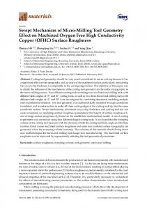
FIG. 1. 共Color兲 Snapshots of damage in a typical cubic lattice system of size L = 64. Number of broken bonds at the peak load and at failure are 114 845 and 126 577, respectively. 共a兲–共i兲 Snapshots of damage after breaking nb number of bonds. The coloring scheme is such that in each snapshot, the bonds broken in the early stages are colored blue, then green, followed by yellow, and finally the last stage of broken bonds are colored red. 共a兲 nb = 50 000, 共b兲 nb = 100 000, 共c兲 nb = 114 845 共peak load兲, 共d兲 nb = 117 000, 共e兲 nb = 119 000, 共f兲 nb = 121 000, 共g兲 nb = 123 000, 共h兲 nb = 125 000, and 共i兲 nb = 126 577 共failure兲.

sizes 共only systems up to L = 24 were considered in 关34,35兴兲 and the method employed for averaging the damage profiles 共see Ref. 关36兴 for a detailed discussion兲. Figure 3 presents the data collapse of the average damage profiles for the damage accumulated between the peak load and failure using a power law scaling. An excellent collapse

FIG. 2. 共Color online兲 Average damage profiles at peak load obtained by first centering the data around the center of mass of the damage and then averaging over different samples.

FIG. 3. 共Color online兲 Data collapse of the average profiles for the damage accumulated between peak load and failure using a power law scaling. The profiles show exponential tails. Data collapse was not achieved using a linear scaling for the localization length. The inset shows the unscaled data of the average profiles, wherein the average has been performed after shifting by the center of mass.

026105-3

PHYSICAL REVIEW E 74, 026105 共2006兲

NUKALA, ZAPPERI, AND ŠIMUNOVIĆ

FIG. 5. 共Color online兲 Crack surface in a typical cubic lattice system of size L = 64. FIG. 4. 共Color online兲 The damage width at peak load and at failure are basically the same. The linear scaling is expected for a uniform distribution and is not due to localization. On the other hand, localization can be observed for postpeak damage, and the width scales as a power law.

of the data is achieved using the scaling form 具⌬p共z,L兲典/具⌬p共0兲典 = f共兩z − L/2兩/␰兲,

共1兲

where the damage peak scales as 具⌬p共0兲典 = L−0.15 and the localization length scales as ␰ ⬃ L␣, with ␣ = 0.50. The damage profiles decay exponentially at large system sizes. We have also tried a simple linear scaling of the form 具⌬p共z , L兲典 / 具⌬p共0兲典 = f关共z − L / 2兲 / L兴, but the collapse of the data is not very good. Similar results have been obtained in the two-dimensional RFM. The postpeak damage profiles display exponential tails; however, the localization length scales as ␰ ⬃ L0.8 关36兴. The diffusive and localization behavior of accumulated damage in the pre- and postpeak regimes can also be inferred from an analysis of the widths of the damage cloud in the pre- and postpeak regimes. The width of the damage cloud is defined as W ⬅ 关具共zb − z¯b兲2典兴1/2, where zb is the z coordinate of a broken bond and the average is taken over different realizations. The measured width of damage cloud at peak load scales as W ⬃ L 共see Fig. 4兲. This result is consistent with the hypothesis that the damage is uniformly distributed 共diffusive兲 at the peak load and localization occurs in the postpeak regime. The uniform distribution of damage at the peak load results in a scaling of the form W ⯝ L / 冑12⬃ 0.288L that is in excellent agreement with the numerical data 共see Fig. 4兲. The width of damage cloud in the postpeak regime scales as W ⬃ L0.7, and this nontrivial scaling exponent indicates that the damage profiles exhibit a localized behavior in the postpeak regime. Another interesting quantity to study is the scaling of the final crack width. Figure 4 indicates that the final crack width scales as W ⬃ L0.5, which is consistent with the scaling of localization length ␰ ⬃ L0.5 used in the data collapse of damage profiles in the postpeak regime. The center of mass shifting of the damage profiles for the purpose of averaging the

damage profiles makes this consistency between the final crack width and the localization length ␰ of the damage profiles self-evident. In addition, this consistency supports the idea that the postpeak damage profile is predominantly due to the localization produced by the catastrophic failure, which at the same time results in the formation of the final crack. Similar behavior is observed in two-dimensional RFM; namely, the width of the damage cloud in the prepeak regime is consistent with the uniform damage profile, and that the scaling of final crack width 共⬃L0.81, see Fig. 11 of Ref. 关36兴兲 is consistent with the scaling of localization length ␰ ⬃ L0.8 共see Fig. 9 of Ref. 关36兴兲 of the postpeak damage profiles. Interestingly, the same consistency in scaling between the final crack width and the localization length of the postpeak damage profiles is observed in the random spring models as well. The final crack width scales as W ⬃ L0.64 共see Ref. 关38兴兲, and the localization length ␰ of the postpeak damage profiles scales as ␰ ⬃ L0.65 共see Fig. 6 of Ref. 关37兴兲. IV. CRACK SURFACE ROUGHNESS

Once the complete fracture of the lattice system has occurred, we identify the final crack by removing the dangling ends and overhangs as shown in Fig. 5. The crack surface is represented by a single valued height function z共x , y兲 in the x − y reference plane, where x 苸 关0 , L兴 and y 苸 关0 , L兴. Several methods have been devised to characterize the roughness of an interface and their reliability has been tested against synthetic data 关39兴. If the interface is self-affine, all the methods should yield the same result in the limit of large samples. For instance, consider the local crack width of a crack line z共x , y = c兲. The local width using the variable bandwidth method is computed as w共ᐉ兲 ⬅ 具兺x关zx − 共1 / ᐉ 兲兺XzX兴2典1/2, where the sums are restricted to windows of length ᐉ along the x direction and the average 具¯典 is taken over all possible origins of the windows along the profile, and over different realizations. The self-affine scaling properties of crack surfaces results in a scaling law of form w共ᐉ兲 ⬃ ᐉ␨ for ᐉ
L that saturates to a value W = w共L兲 ⬃ L␨ corresponding to the global width. A more precise value of the exponents is obtained from the power spectrum, which is expected to

026105-4

PHYSICAL REVIEW E 74, 026105 共2006兲

CRACK SURFACE ROUGHNESS IN THREE-¼

FIG. 7. 共Color online兲 The collapse of the local crack widths in the x direction with ␨ = 0.52. The collapse of the data, however, is not very good. The scenario for the collapse of local crack widths in y direction is similar.

FIG. 6. 共Color online兲 The local width w共l兲 of the crack in the x and y directions for different lattice sizes in log-log scale. The crack width scaling in x and y directions is identical. The global width yields a scaling exponent ␨ = 0.52.

yield more precise estimates 关39兴. The power spectrum or the structure factor is computed as S共k兲 ⬅ 具zˆkzˆ−k典 / L, where zˆk ⬅ 兺xzx exp共2␲ixk / L兲, and decays as S共k兲 ⬃ k−共2␨+1兲. We estimate the crack surface roughness in the x and y directions by considering number of slices along each direction. For instance, the crack roughness in the x direction is computed by considering the roughness of L + 1 number of slices, each with z共x , y = c兲, where c is a constant that takes on values c = 1 , 2 , . . . , L + 1. Once the crack line roughness of each of these L + 1 lines with z共x , y = c兲 is computed, the crack surface roughness in the x direction is estimated as the average roughness of these L + 1 crack lines, which is then averaged over different realizations. Similarly, the crack surface roughness in the y direction is computed as the average roughness of the L + 1 crack lines z共x = c , y兲, where c is a constant that takes on values c = 1 , 2 , . . . , L + 1 for each of the L + 1 slices, respectively. Figure 6 presents the scaling of local crack width in the x and y directions for different lattice system sizes. The results presented in Figs. 6共a兲 and 6共b兲 indicate that the crack width scaling in the x and y directions is identical.

A reference line, obtained by fitting the scaling of the global width with L, indicates a roughness exponent ␨ = 0.52. We have obtained the same scaling exponents in both x and y directions. It should be noted that the exponent ␨ = 0.52 differs slightly from the global crack width exponent of ␨ = 0.5 presented in Fig. 4. The reason for this discrepancy is that the crack width exponent in Fig. 4 is calculated as W = 具兺共z −¯兲 z 2典1/2 for the entire crack surface z共x , y兲, whereas the global width exponent in Fig. 6 is averaged over L + 1 crack lines of z共x , y = c兲 with c = 1 , 2 , . . . , L + 1. It should also be noted that the exponent ␨ = 0.52 differs considerably from the exponent ␨ = 0.62± 0.05 proposed in 关27,34,35兴 and that of ␨ = 0.41± 0.02 proposed in 关29兴. However, the difference may be due to the fewer number of statistical samples considered in these earlier studies. A direct fit of the local width based on Figs. 6共a兲 and 6共b兲 would not be reliable due to the very small scaling regime. Thus, in Fig. 7 we present the collapse of the local crack width data using the scaling form w共ᐉ兲 ⬃ ᐉ␨ f共ᐉ / L兲 and the result is not very good. In two-dimensional RFM, our data with improved statistics and large system sizes 关22兴 indicated that the crack roughness scaling is anomalous 关9兴. In previous measurements on two-dimensional RFM, anomalous scaling could not be detected since the data was available only for smaller system sizes. Anomalous scaling has been observed not only in various growth models 关9兴 but also in fracture surfaces in granite 关10兴 and wood samples 关11兴. Anomalous scaling implies that the exponent describing the system size dependence of the surface differs from the local exponent measured for a fixed system size L. In particular, the local width scales as w共ᐉ兲 ⬃ ᐉ␨locL␨−␨loc, so that the global roughness W scales as L␨ with ␨ ⬎ ␨loc. Consequently, the power spectrum scales as S共k兲 ⬃ k−共2␨loc+1兲L2共␨−␨loc兲. The upward shift of the w共ᐉ兲 presented in Figs. 6共a兲 and 6共b兲 for different system sizes is a fingerprint of anomalous scaling, since such a shift indicates that w共ᐉ兲 grows with L. This is a key feature of anomalous scaling that can be spotted by just looking at the

026105-5

PHYSICAL REVIEW E 74, 026105 共2006兲

NUKALA, ZAPPERI, AND ŠIMUNOVIĆ

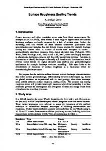
FIG. 8. 共Color online兲 The power spectrum of the crack S共k , L兲 in x direction for different lattice sizes in log-log scale. 共a兲 Uncollapsed power spectrum data. The collapse of the data is not perfect, and the slope of the spectra is equal to −1.80. A line with a slope of −共2␨ + 1兲 = −2.0 is provided for reference. 共b兲 The spectra for all of the different lattice sizes can be collapsed by normalizing S共k , L兲 with L2共␨−␨loc兲, where 共␨ − ␨loc兲 = 0.1. The slope defines the local exponent as −共2␨loc + 1兲 and is equal to −1.80, implying that ␨loc = 0.4 and ␨ = 0.5. Identical exponents are obtained using the power spectrum data in y direction.

local roughness amplitudes. In order to further check the presence of anomalous scaling in three dimensions, we report in Figs. 8共a兲 and 8共b兲 the x-direction data collapse of the power spectra for different system sizes. Identical results are obtained using the power-spectrum data in the y direction. Figure 8共a兲 presents the uncollapsed power spectrum data and two reference lines with slopes of −共2␨loc + 1兲 = −1.8 and −共2␨ + 1兲 = −2.0. Clearly, the collapse of the data in Fig. 8共a兲 is not perfect; there appear to be small but systematic shifts in the data with system sizes. Also, the reference line with a slope of −共2␨ + 1兲 = −2.0 共corresponding to a global roughness exponent of ␨ = 0.5兲 is not a good fit, which suggests the presence of anomalous scaling. On the other hand, a perfect

FIG. 9. 共Color online兲 Crack width distributions for different lattice sizes. 共a兲 Deviations are observed from the scaling form P共W2兲 = P共W2 / 具W2典兲. 共b兲 The collapsed distribution of crack widths ln共W2兲−␩W2 . obtained using the reduced variable ¯␰ 2 = W

␨ W2

data collapse is obtained in Fig. 8共b兲 using the anomalous scaling form S共k兲 ⬃ k−共2␨loc+1兲L2共␨−␨loc兲, with ␨ − ␨loc = 0.1. A straight line fit of the power law decay of the spectrum yields an estimate for the local roughness exponent equal to ␨loc = 0.4, which implies a global roughness exponent of ␨ = 0.5, since ␨ − ␨loc = 0.1. Clearly, the global roughness exponents obtained using the variable bandwidth method 共0.52兲 and the power spectrum method 共0.5兲 are in excellent agreement, and the small difference can be attributed to the bias associated to the methods employed 关39兴. Although the value of ␨ − ␨loc as estimated using the power spectrum method is small, it is significantly larger than zero and it may even correspond to a logarithmic growth. However, based on our numerical results, which included lattice system sizes up to L = 64 with extensive statistical sampling, it is not possible to conclude with certainty whether anomalous scaling of crack surface roughness is present in threedimensional RFM or not. Simulations on much larger lattice systems are anticipated to clarify this.

026105-6

PHYSICAL REVIEW E 74, 026105 共2006兲

CRACK SURFACE ROUGHNESS IN THREE-¼

normal distribution for the crack global width distribution. Finally, in Ref. 关22兴, it is shown that the crack width distributions in the two-dimensional RFM are also well fit by a log-normal distribution for both diamond and triangular lattices of different system sizes. The data collapse and lognormality of crack width distributions in three-dimensional RFM as well as in two-dimensional RFM for different lattice topologies suggests universality of crack width distributions. VI. CONCLUSIONS

FIG. 10. 共Color online兲 The collapse of the crack width distribution data onto a straight line suggests that it follows a lognormal distribution. The inset shows that a Gaussian distribution is not an adequate fit for the crack width distribution. V. CRACK WIDTH DISTRIBUTION

We have analyzed the probability density distribution p共W2兲 of the global crack width. This distribution has been measured for various interfaces in models and experiments and typically rescales as 关40兴 p共W2兲 = p共W2/具W2典兲/具W2典,

共2兲

where 具W2典 ⬃ L2␨ is the average global width. Equation 共2兲 implies that the corresponding cumulative distribution P共W2兲 of crack global width scales as P共W2兲 = P共W2 / 具W2典兲. Figure 9共a兲 shows that a reasonable collapse of the crack global width distributions for different lattice system sizes may be achieved using Eq. 共2兲. However, the data collapse is not perfect, and deviations from the scaling P共W2兲 = P共W2 / 具W2典兲 are evident. Alternatively, an excellent collapse of the data is obtained in Fig. 9共b兲 using the reduced ln共W2兲−␩W2 , where ␩ 2 and ␨ 2 delog-normal coordinate ¯␰ 2 = W

␨ W2

W

W

note the mean and standard deviation of logarithm of W2. In Fig. 10, a reparametrized form of the log-normal distribution is presented. The collapse of the data onto a straight line indicates that the log-normal distribution represents an excellent fit to the distribution of crack global widths. We have also tried a Gaussian fit for the distribution of crack global widths. The inset of Fig. 10 presents a Gaussian fit for the crack global widths distribution wherein significant curvature in the collapsed plots can be observed. This suggests that the normal distribution is not as good a fit as the log-

In this paper we have analyzed the localization properties of fracture in the three-dimensional random fuse model using an improved statistical sampling and larger lattices than what was previously done in the past. We have analyzed the roughness of the final crack and found a local exponent ␨loc = 0.4, which is slightly different from the global roughness exponent ␨ = 0.52. A similar difference between local and global exponents was also found in two-dimensional simulations for both triangular and diamond lattices 关22兴, suggesting that anomalous scaling is a generic feature of the fracture of disordered media, as already found in fracture experiments 关10兴. The numerical value of the exponents is, however, quite far from the three-dimensional experimental results, indicating that additional physical mechanisms should probably be taken into account. We have also evaluated the width distribution 关40兴 that can be collapsed into a single curve for different lattice sizes and it appears to be well fit by a lognormal distribution. Finally, the analysis of damage profiles indicates that the localization process occurs abruptly after peak load. In summary, the present results seem to indicate that the RFM provides only a qualitative description of the fracture surface morphology found in experiments. The quantitative differences may be attributed to the strong simplifications present in the model such as its scalar nature, the quasistatic dynamics, and the absence of a pre-existing notch; although a roughness exponent of ␨ = 0.5 关30兴 is obtained using threedimensional Born model as well. On the other hand, the initial phase of damage accumulation leading to localization and failure in a strongly disordered sample are well captured by the RFM model, but further work is needed to clarify these issues. ACKNOWLEDGMENTS

This research is sponsored by the Mathematical, Information and Computational Sciences Division, Office of Advanced Scientific Computing Research, U.S. Department of Energy, under contract number DE-AC05-00OR22725 with UT-Battelle, LLC. S.Z. is thankful for hospitality provided by the Kavli Institute for Theoretical Physics where this work was completed and also acknowledges partial financial support through NSF Grant No. PHY99-07949.

026105-7

PHYSICAL REVIEW E 74, 026105 共2006兲

NUKALA, ZAPPERI, AND ŠIMUNOVIĆ 关1兴 Statistical Models for the Fracture of Disordered Media, edited by H. J. Herrmann and S. Roux 共North-Holland, Amsterdam, 1990兲; Non-Linearity and Breakdown in Soft Condensed Matter, edited by K. K. Bardhan, B. K. Chakrabarti, and A. Hansen 共Springer Verlag, Berlin, 1994兲; B. K. Chakrabarti and L. G. Benguigui, Statistical Physics of Fracture and Breakdown in Disordered Systems 共Oxford University Press, Oxford, 1997兲. D.Krajcinovic and van Mier, Damage and Fracture of Disordered Materials 共Springer Verlag, New York, 2000兲. 关2兴 B. B. Mandelbrot, D. E. Passoja, and A. J. Paullay, Nature 共London兲 308, 721 共1984兲. 关3兴 B. B. Mandelbrot, Phys. Scr. 32, 257 共1985兲. 关4兴 For a review, see E. Bouchaud, J. Phys.: Condens. Matter 9, 4319 共1997兲; E. Bouchaud, Surf. Rev. Lett. 10, 73 共2003兲. 关5兴 K. J. Maloy, A. Hansen, E. L. Hinrichsen, and S. Roux, Phys. Rev. Lett. 68, 213 共1992兲; E. Bouchaud, G. Lapasset, J. Planés, and S. Navéos, Phys. Rev. B 48, 2917 共1993兲. 关6兴 P. Daguier, B. Nghiem, E. Bouchaud, and F. Creuzet, Phys. Rev. Lett. 78, 1062 共1997兲. 关7兴 J. Schmittbuhl, S. Roux, and Y. Berthaud, Europhys. Lett. 28, 585 共1994兲; J. Schmittbuhl, F. Schmitt, and C. Scholz, J. Geophys. Res. 100, 5953 共1995兲. 关8兴 J. J. Mecholsky, D. E. Passoja, and K. S. Feinberg-Ringel, J. Am. Ceram. Soc. 72, 60 共1989兲. 关9兴 J. M. López, M. A. Rodríguez, and R. Cuerno, Phys. Rev. E 56, 3993 共1997兲. 关10兴 J. M. López and J. Schmittbuhl, Phys. Rev. E 57, 6405 共1998兲. 关11兴 S. Morel, J. Schmittbuhl, J. M. López, and G. Valentin, Phys. Rev. E 58, 6999 共1998兲. 关12兴 L. de Arcangelis, S. Redner, and H. J. Herrmann, J. Phys. 共Paris兲, Lett. 46, 585 共1985兲. 关13兴 M. Sahimi and J. D. Goddard, Phys. Rev. B 33, 7848 共1986兲. 关14兴 B. Kahng, G. G. Batrouni, S. Redner, L. de Arcangelis, and H. J. Herrmann, Phys. Rev. B 37, 7625 共1988兲. 关15兴 L. de Arcangelis, A. Hansen, H. J. Herrmann, and S. Roux, Phys. Rev. B 40, 877 共1989兲. 关16兴 A. Delaplace, G. Pijaudier-Cabot, and S. Roux, J. Mech. Phys. Solids 44, 99 共1996兲. 关17兴 S. Zapperi, P. Ray, H. E. Stanley, and A. Vespignani, Phys. Rev. Lett. 78, 1408 共1997兲; Phys. Rev. E 59, 5049 共1999兲. 关18兴 A. Hansen and S. Roux, in Damage and Fracture of Disordered Materials, edited by D. Krajcinovic and van Mier 共Springer Verlag, New York, 2000兲 pp. 17–101. 关19兴 A. Hansen, E. L. Hinrichsen, and S. Roux, Phys. Rev. Lett. 66, 2476 共1991兲. 关20兴 E. T. Seppälä, V. I. Räisänen, and M. J. Alava, Phys. Rev. E 61, 6312 共2000兲. 关21兴 J. O. H. Bakke, J. Bjelland, T. Ramstad, T. Stranden, A.

Hansen, and J. Schmittbuhl, Phys. Scr. T106, 65 共2003兲. 关22兴 S. Zapperi, P. K. V. V. Nukala, and S. Simunovic, Phys. Rev. E 71, 026106 共2005兲. 关23兴 G. Mourot, S. Morel, E. Bouchaud, and G. Valentin, Phys. Rev. E 71, 016136 共2005兲. 关24兴 C. Poirier, M. Ammi, D. Bideau, and J. P. Troadec, Phys. Rev. Lett. 68, 216 共1992兲. 关25兴 T. Engoy, K. J. Maloy, A. Hansen, and S. Roux, Phys. Rev. Lett. 73, 834 共1994兲. 关26兴 J. Kertész, V. K. Horváth, and F. Weber, Fractals 1, 67 共1993兲; J. Rosti, L. I. Salminen, E. T. Seppälä, M. J. Alava, and K. J. Niskanen, Eur. Phys. J. B 19, 259 共2001兲; L. I. Salminen, M. J. Alava, and K. J. Niskanen, Eur. Phys. J. B 32, 369 共2003兲. 关27兴 G. G. Batrouni and A. Hansen, Phys. Rev. Lett. 80, 325 共1998兲. 关28兴 V. I. Räisänen, M. J. Alava, and R. M. Nieminen, Phys. Rev. B 58, 14288 共1998兲. 关29兴 V. I. Räisänen, E. T. Seppälä, M. J. Alava, and P. M. Duxbury, Phys. Rev. Lett. 80, 329 共1998兲. 关30兴 A. Parisi, G. Caldarelli, and L. Pietronero, Europhys. Lett. 52, 304 共2000兲. 关31兴 A. Hansen, E. L. Hinrichsen, and S. Roux, Phys. Rev. B 43, 665 共1991兲. 关32兴 P. K. V. V. Nukala and S. Simunovic, J. Phys. A 36, 11403 共2003兲. 关33兴 P. K. V. V. Nukala and S. Simunovic, J. Phys. A 37, 2093 共2003兲. 关34兴 A. Hansen and J. Schmittbuhl, Phys. Rev. Lett. 90, 045504 共2003兲. 关35兴 T. Ramstad, J. O. H. Bakke, J. Bjelland, T. Stranden, and A. Hansen, Phys. Rev. E 70, 036123 共2004兲. 关36兴 P. K. V. V. Nukala, S. Simunovic, and S. Zapperi, J. Stat. Mech.: Theory Exp. 2004, P08001. 关37兴 P. K. V. V. Nukala, S. Zapperi, and S. Simunovic, Phys. Rev. E 71, 066106 共2005兲. 关38兴 G. Caldarelli, R. Cafiero, and A. Gabrielli, Phys. Rev. E 57, 3878 共1998兲. 关39兴 J. Schmittbuhl, J. P. Vilotte, and S. Roux, Phys. Rev. E 51, 131 共1995兲. 关40兴 G. Foltin, K. Oerding, Z. Rácz, R. L. Workman, and R. K. P. Zia, Phys. Rev. E 50, R639 共1994兲; M. Plischke, Z. Rácz, and R. K. P. Zia, Phys. Rev. E 50, 3589 共1994兲; Z. Rácz and M. Plischke, Phys. Rev. E 50, 3530 共1994兲; T. Antal, M. Droz, G. Györgyi, and Z. Rácz, Phys. Rev. Lett. 87, 240601 共2001兲; T. Antal, M. Droz, G. Györgyi, and Z. Rácz, Phys. Rev. E 65, 046140 共2002兲; A. Rosso, W. Krauth, P. Le Doussal, J. Vannimenus, and K. J. Wiese, Phys. Rev. E 68, 036128 共2003兲.

026105-8