Data-Centric Storage in Wireless Sensor Network

Data-Centric Storage in Wireless Sensor Network Khandakar Ahmed*, Mark Gregory School of Electrical and Computer Engineering RMIT University, Melbourne, Australia *[email protected] Abstract Distributed Data-Centric Storage is considered to be a promising and efficient approach for data storage and search mechanism. Since External Storage (ES) and Local Storage (LS) mechanisms often lead to high energy consumption, latency and creation of hotspot, DCS becomes preferable alternative approach for large scale wireless sensor networks (WSNs). Since 2002, many potential research works are conducted in this field focusing DCS routing, multi-replication, similarity search, range queries, multi-attribute event, non-uniformity of sensor network etc. In this chapter a comprehensive state-ofthe-art study is provided in which the prime focus of WSN DCS mechanism, design guidelines that inspired these methods, drawbacks and shortcomings of the existing solutions are thoroughly exposed.

1. Introduction Wireless Sensor Network is an emerging technology suitable for unattended monitoring of a straddling infrastructure (such as industries, factories, bridges etc.), wide range of environments and even in humans. WSN, along with mobile ad-hoc network, is one of the research trends in the field of infrastructure-less wireless networks. Both mobile ad-hoc and WSN is highly infrastructure-less with dynamic nature of nodes and their unpredicted mobility pattern. However unlike mobile ad-hoc, in WSN limited resources and extremely large number of nodes are two major challenges. WSN is mainly application specific and data-centric. The identity of a sensor is not as important as the data associated with it. Data Storage and retrieval methods in WSN can be classified into three canonical approaches [1-2]: External Storage (ES), Local Storage (LS) and Data-Centric Storage (DCS). In ES [3-6] nodes send data to the base station or gateway without waiting for any query. Nodes inside the network or any user outside the network sends query to the base station. This may create bottleneck to the base station. This also waste energy when every single data are sent to the base station without aggregation. In LS [7-11], each node keeps its sensed data locally and uses flooding for query consuming a significant amount of energy resources. In DCS [12-15], it is proposed to choose one (or more) rendezvous node (s), based on the event type, as the target node to store data. This reduces both storage and query cost. The first DCS is Geographic Hash Table (GHT) proposed in 2002. Since then, lot of research has been done targeting different challenges: non-uniformity of the network, multi-dimensional attribute, range query, data aggregation and similarity search. However, none of the works covers all these issues together though different proposals try to give solutions to different problems. In this chapter, most of the wellaccepted proposed DCS techniques are presented providing a clear and in-depth literature to the researcher and student of this field. The rest of this chapter is organized as follows: some major challenges relevant to DCS are discussed in section 2. Section 3 briefly discusses most relevant works studying DCS, classified into two major routing categories: point-to-point routing (section 3.1) and routing based on tree-structures (section 3.2), in the literature and presents their main contribution and rationale based on the challenges mentioned in section 2. Section 4 concludes and provides a comparative table highlighting salient features of each DCS mechanism.

2. Challenges 2.1. Multi-dimensional Attribute The recent technological development in WSN is the heterogeneity of sensors, where the sensor may have multiple capabilities in terms of computing, power supplies, communicating and sensing [16-17]. Hence, a heterogeneous network at present is able to detect multiple types of attributes such as – humidity, temperature, level of particular gas in atmosphere etc. For example- in an air pollution

measuring application, the measurement data may be the fusion of several parameters such as temperature, level of carbon monoxide, level of smoke etc. In such application, it is obvious to have storage and search mechanism for multi-dimensional queries. In [13, 18-19], authors propose multi-dimensional storage and query mechanism for DCS.

2.2. Range versus Point Queries Range query is another challenge for DCS scheme. For example, a user may interest on a particular range rather than on specific point value. Say, air pollution may be encountered if the level of carbon monoxide is in the range between 30 L/mol and 90L/mol. So, a possible query is to find all the sensing point where the level of carbon monoxide falls in the above stated range. Using range queries, users can drill down their search efficiently for the events of interest. The query presented above illustrates this, where an environmental scientist, on a particular forest, is presumably interested in discovering above stated range of carbon monoxide and perhaps also wants to map it with some other parameters to take certain action or draw a conclusion [13]. In [13, 18-22], authors implement range query mechanism in different format. Y. Chung et al. [21] mainly propose an efficient technique for similarity search in DCS which works for both point and range query. X. Li, et al. also show both point and range query in their multidimensional DCS model. [19] provides a model called Distributed Spatial Temporal Similarity Data Storage, referred as SDS, technique which supports range query. DIFS [20] performs data fusion based on conveyance of data through the network. The routing is designed on top of quad tree in a manner that balances communication load across the index and the range is maintained along the hierarchy of sensor nodes.

2.3. Similarity Search Due to the imprecision of sensor hardware and variation of environmental parameters, the similarity search problem in WSN received tremendous attention. Moreover, in certain application or circumstances in addition to exact match it is necessary to search within a specified similarity range. For example, a multi-dimensional query on attributes temperature, carbon monoxide, forest name, location, smoke level with value 1000| 150 L/mol| Melaleuca| North| 130 L/mol may also interest on similar set of value 900| 150 L/mol| Melaleuca| South| 130 L/mol. Similarity search may also be useful in many application such as finding similar flow patterns in ocean or wildlife activity patterns in habitat monitoring [19]. Traditional approach of similarity search is improper and inefficient for the highly energy-constraint sensor network. It is necessary to search similar data to the query without collecting data from all sensors. [19, 21] are two DCS mechanisms implementing efficient technique for similarity search. [19] implements similarity search with low energy consumption by assigning weight to the different attributes based on their importance. In contrast, [21] maintains two variables for maintaining range in the index node of each zone, network is divided into zones based on the concept of Hilbert curve, and uses three different functions referred as backward, forward and bi-direction probing to search similar data.

2.4. Data Aggregation Based on the basic data stored in sensors, DCS networks can facilitate data aggregation in a fully distributed way. By using data aggregation, traffic generated by producer nodes can be reduced before answering consumer queries. Monitoring building integrity during earthquakes by engineers, habitat monitoring by biologists, monitoring temperature and power usage in data centers by cluster computer administrator are examples of sensor applications depending on the ability to extract summary (aggregate) data rather than raw data from the network. In DCS, replicas can be ideally used for data aggregation as they receive all the data from the producers in its surrounding area. However, there are many form of data aggregation implementation. TinyDB [23], madwise [24] and TAG [9] are some of the aggregation mechanism proposed mainly for WSN database. They can be adapted to DCS networks as well. In [25], Cuevas et al. model data aggregation in multi-replication DCS systems for Wireless Sensor and Actor Networks (WSAN). DIFS [20] and Resilient Data Centric Storage [22] in WSN also provide data aggregation in DCS mechanism.

2.5. Non-uniformity of Sensor Network Field In every deployments, sensor may not be uniformly distributed which means some sections/zoned are may be densely populated while other may be not. Moreover, in mobile WSN, sensors may move from one place to another creating non-uniformity later. In current state of art, most DCS schemes are proposed considering that sensors are uniformly distributed. This assumption leads to data losses in overburdened sensors. Load Balanced Data Centric Storage (LB-DCS) [26] deals with non-uniformity based on two mechanism. At first it estimates network distribution and then exploits data dissemination method based on the estimation.

2.6. Multi-replication Multi-replication reduces the data loss that happens due to node failure or its mobility from one rendezvous zone to another. Furthermore, multi-replication may facilitate data fusion and aggregation. GHT [1] is the first which proposes multi-replication using PRP in order to replicate data. It also extends GHT to SR-GHT [1] to avoid creation of hotspot in home node, where the number of replicas is Nr = 4d. However, the most interesting issue is it never replicates data to all of its replica nodes rather the producer node stores data only to its closest replica and a query node needs to query all the replica nodes. Tug-of-War [27] implements the same replication mechanism based on 4d grid. Like SR-GHT and Tug-of-War, Quadratic Adaptive Replication [28] uses the same grid based replication mechanism. However, the number of replicas in QAR follows a more adaptable quadratic evolution Nr = d2 and it also allows selecting the optimal number of replicas from wider set of values.

2.7. Balancing the Storage It is important to balance the storage load among the sensor to prevent imposing too high of a storage load creating hotspot on some nodes. Load Balancing is implemented in [19, 26, 29-30]. In SDS [19], a N

zone head estimates its storage usage status using

∑S i =1

i

N

. After receiving storage request, each zone

head first examines if its zone storage usage has reached threshold, denoted by ϕ , or not. If so, the head redirects the storage request to neighbour zone keeping a pointer to it. [29] uses cover-up scheme to balance the load inside a zone. LB-DCS [26] balances the load in similar fashion like SDS [19] by estimating the zone density. However, unlike SDS, LB-DCS estimates zone density using the number of sensor nodes and then disseminates this density information through out the network.

3. DCS Mechanisms: In the current state of the art, DCS can be classified based on two types of routing referred as: point-topoint routing and routing relies on tree-construction technique. The former method deterministically map the name of an event (e) to the routable address (i) associated with a particular node. In contrast, the later method relies on tree-construction technique. It divides the whole network into a tree structure and provides mapping of data toward paths with minimal assumption about the underlying infrastructure.

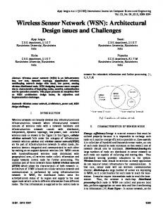
3.1. DCS Mechanisms Based on Point-to-Point Routing 3.1.1. Geographic Hash Table Authors in [1] are the pioneer in providing the noble concept of Data Centric Storage (DCS) scheme in 2002. The motivation of their wok is to make effective use of the vast amount of data gathered by large scale sensor network using scalable, self-organizing and energy-efficient data dissemination algorithms. Authors use Distributed Hash Table (DHT) [31-33] in order to hash keys, for example event name or type, into geographic co-ordinates and store this event to sensor nodes in a geographic location closer to these co-ordinates. Greedless Perimeter Stateless Routing (GPSR) [34] is used to store and/or retrieve data to/from a sensor node. GHT [1] uses a hash function over the event name, say humidity, and to find a corresponding key. When a sensor node senses an event, it is mapped to the corresponding key based on the event name. GHT then uses put (k, d), k – hash key used as destined geographical location and d - data, function which forwards this packet to the k location using GPSR. The closest sensor node to the geographical

location (k) is chosen as the home node, which stores the data, for this event type. Similarly, when consumer wants to consume/query a data of an event type (for this particular case e.g. humidity), GHT again maps event type to hash key (k) and uses get(k) to forward the query to the corresponding spatial/geographical location (k). The home node then replies by providing stored data for that event type. In Figure 1, sensors are represented by ‘ ’. A producer node senses a value and forwards it to home node denoted by ‘ ’. In turn, another consumer node uses same hash function and retrieves the stored data from the home node. In storing process, represented by ‘ ’, producer node sends data to the target node while in retrieval process, denoted by ‘ ’, query is first forwarded to home node and replies is then sent back to consumer. Home Node

Producer Node: d = sensed value k = DHT (‘humidity’) put (k, d)

Consumer Node: k = DHT (‘humidity’) get (k)

Figure 1. Geographic Hash Table

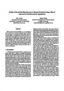
3.1.1.1. Routing Algorithm GHT uses two types of routing algorithm: GPSR and Perimeter Refresh Routing (PRP). GPSR is used to route packets geographically while PRP is used to accomplish replication of key-value pairs and consistent replacement at the appropriate home nodes when the network topology changes. There are two distinct algorithm that GPSR uses for routing- firstly, a greedy forwarding algorithm [35] that moves packets progressively closer to the destination at each hop and secondly a perimeter forwarding algorithm that forwards packets where greedy forwarding is impossible. In greedy forwarding rule, a node s forwards a packet to its neighbour x which is closest to the destination (see Figure 2(a)). However, greedy forwarding fails when no neighbour is closer than S to the destination. GPSR uses perimeter routing algorithm to recover from this void condition. In Figure 2(b), there is no neighbour in the range of S which is closer to the destination D than S. In such situation, perimeter forwarding uses right hand rule. Figure 2(c) illustrates right hand rule. GPSR starts with greedy forwarding rule but switches to perimeter forwarding when greedy fails. GPSR again returns to greedy from perimeter-mode when the packet reaches a node closest to destination than that at which GPSR enters into perimeter forwarding.

2.

x

S

y

D

X

3.

1. z (a)

(b)

(c)

Figure 2. (a) Greedy forwarding routing (b) x has no neighbour closer to D than itself (c) Packets travel clockwise around enclosed region [1]

3.1.1.2. Evaluation In GHT [1], authors uses a simple analytical method to compare the performance of GHT with two other canonical methods: External Storage (ES) and Local Storage (LS). It is considered that, the deployed sensor network has n sensor nodes enable to detect T event types. Dtotal denotes the total number of events detected, Q denotes the number of event types for which query is made and Dq denotes the total number of successful response found for Q queries. So, the costs are (list indicates full listing of events is returned while summary indicates only summary of events is returned): External Storage:

Total : Dtotal n Hotspot : Dtotal Local Storage:

Total : Qn + Dq n Hotspot : Q + Dq Data-Centric Storage:

Total : Q n + Dtota n + Dq n (list )

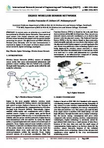
Total : Q n + Dtotal n + Q n ( summary ) Hotspot : Q + Dq (list )or 2Q (summary ) 3.1.1.3. Multi-Replication A home node becomes a hotspot if too many events with the same key are detected. To address this issue authors have extended GHT by employing Structured Replication (SR). Structured Replication introduces a hierarchical scheme where one can have 4d – 1 mirror images of the root home node.

Root point: (3, 3) Level 1 point: (53, 3), (3, 53), (53, 53) Level 2 mirror point: (28, 3), (3, 28), (28, 28), (78, 3), (53, 28), (78, 28), (3, 78), (28, 53), (28, 78), (78, 53) (53, 78), (78, 78)

Figure 3. Structured Replication [1] Here, d denotes the depth of hierarchy. As shown in Figure 3, a decomposition of two levels (d=2) is deployed having 42 – 1 (15) mirror images at different levels. A producer node can store the detected event to its closest mirror node reducing the storage cost to

 n O d  from O n . In retrieval phase, 2 

( )

GHT needs to forward query to all mirror images. The query is first forwarded to root node which is then forwarded to all mirror images in level 1 and then level-one nodes forward this query to level 2

mirror images. This again increases the retrieval cost to

 n O 2 d n from O d  . Thus, for an event 2 

(

)

with Di detected instances and Qi queries the total cost for storing and retrieval of this event is approximated as:

  n  O Qi 2 d n + Di  d   .    2  

3.1.1.4. Discussion Use of single home node could create a hot spot as all the traffic targets a single node for particular event type consuming its energy quicker than others. However, to solve this problem local replication is done by means of PRP. This works fine at certain extent as several replicas can answer the consumer queries by balancing load among them. However, for popular event many queries may reach the home perimeter thus PRP creating routing hotspot surrounding the home node. GHT doesn’t address multidimension, range query, non-uniformity, aggregation and similarity search.

3.1.2. Data Storage and Range Query Mechanism for Multi-dimensional Attributes The paper [18] proposes an energy-efficient & scalable multi-dimensional range query mechanism (MDAs) to retrieve data. It builds an in-network distributed data structure by mapping multidimensional attributes to their corresponding range spaces. Authors consider few assumptions prior to start their work: 1) The sensors are uniformly and densely deployed 2) each node can sense multiple events iii) each node maintains a neighbour table via periodic beacon message exchanges and knows its own geographic location. A source node detects an event with a set of attribute values, E = {a1, a2... an}. It is assumed that all attributes value is scalar and is normalized to (0-1). An event is assigned with k bit code where k=2m. If 0 < a i < 0.5 , the ith bit code is assigned to 0 otherwise 1. For xj=a2j-1 and yj=a2j attribute values of E is assigned a serial bit code B = {x1, y1, x2, y2……xm, ym}. For example, an event E = {0.8,0.7,0.4,0.3} is assigned a four bit code B={ x1, y1, x2, y2}={1,1,0,0}. Assignment of code B can be achieved through following: ( 0 < a i < 0.5 and 0.5 < ai < 1 are generalized to

0 < 2ai < 1 and 1 < 2a i < 2 respectively)

Bˆ = [a1 , a 2 ,........., a 2 m ]2 I k = [2a1 ,2a 2 ,.......,2a 2 m ]

B = [ 2a1 , 2a 2 ,......2a 2 m ] = [ x1 , y1 , x 2 , y 2 ......., x m , y m ] This code B is mapped to a range space R

= [ xlow − xup , ylow − y up ] . Hence, it is important to

calculate (xlow, ylow) and (xup, yup) to find range space R. In code B, x = x1, x2… xm are used to calculate X of R and y = y1, y2… ym are used to calculate Y of R. In code B, if x1=1 its value is in between 0.5 and 1; if x2=1 its value is in between 0.5 and 0.5+(0.5)2. So, Xlow = x1(0.5)+x2(0.5)2+……. + xm(0.5)m. Similarly Ylow = y1(0.5)+y2(0.5)2+……. + ym(0.5)m. This is generalized to:

M kx 2

 (0.5)1   0  (0.5) 2  0 =  M   M (0.5) k 2   0

  (0.5)  0   (0.5) 2  M   M  0  k  (0.5) 2  0

1

Rlow = [ xlow , y low ] = B × M

Hence, Again, Xup is defined by:

Xup= 1 – (x1(0.5) +x2(0.5)2 +……. + xm(0.5)m) So,

&& = B ⊕ J B k

J k = [1,1,......,1]1×k So,

&& × M Rˆ up = [ xˆ up , yˆ up ] = B Rup = [ xup , y up ] = J 2 − Rˆ up

So,

R = [ xlow − xup , ylow − y up ]

Example:

Bˆ = [0.8,0.7,0.4,0.7,0.3,0.6] × 2 I 6 = [1.6,1.4,0.8,1.4,0.6,1.2] = [ 1.6, 1.4, 0.8, 1.4, 0.6, 1.2] = [1,1,0,1,0,1]

Rlow = B × M 6×2

 (0.5)1   0 (0.5) 2 = [1,1,0,1,0,1] ×   0 (0.5) 3   0 = [0.5,0.875]

&& = B ⊕ J = [1,1,0,1,0,1] ⊕ [1,1,1,1,1,1] B 6 = [0,0,1,0,1,0]

&& × M = [0.375,0] Rˆ up = B

0   (0.5)1  0   (0.5) 2  0   (0.5) 3 

Rup = [ xup , yup ] = J 2 − Rup = [1,1] − [0.375,0] = [0.625,1] Hence, the range space is defined by R

= (0.5 − 0.625,0.875 − 1) . Figure 4 illustrates the MDAs

storage and query process. For routing GPSR (refer to section 3.1.1.1) is used. Range Space: {0.5-0.625, 0.875-1} 1

0.875

E = {0.6, 0.8, 0.3, 0.7, 0.1 0.9}

E = {0.8, 0.7, 0.4, 0.7, 0.3 0.6}

0.5

0

0.625

0

1

Figure 4. Multidimensional Range Query Mechanism (MDAs) [18]

3.1.2.1. Simulation and Evaluation The algorithm is simulated and compared with another range query scheme namely multi-dimensional data (DIM) [13]. Authors evaluates MDAs again DIM firstly for average message cost with insertion and queries and secondly for number of dropped events in exchange for the quality of data. It is shown that in every case MDAs outperforms DIM 3.1.2.2. Discussion One of the major limitations of this DCS mechanism is consideration of uniform distribution of sensor nodes. It is very likely to have node failure in large scale deployed networks with massive number of sensor nodes. This work is highly inclined to data loss due to its no replication policy. It is also not suitable for range query, data aggregation, similarity search and obviously non-uniform network distribution. However, simple and efficient rendezvous node selection procedure makes this work attractive among many other DCS mechanisms.

3.1.3. Distributed Spatial-Temporal Data Storage Scheme Similarity Data Storage (SDS) [19] proposes an efficient spatial-temporal similarity data storage scheme for both static and dynamic Wireless Sensor Network (WSN). Efficient aggregation and query of data, similarity search for multi-attribute data and spatial temporal search are identified as three major challenges faced by data centric storage schemes. SDS is claimed to be unique by authors in its spatial-temporal functionality and similarity search functionalities. It aims to reduce overhead, energy consumption and searching latency. In SDS, a deployed large-scale WSN field is considered as a rectangular field. The entire field is divided into small rectangular zones. Each zone has a dedicated sensor node named as zone head. It is assumed that each node in the network is configured with three basic information: 1) Number of zones horizontally nx and vertically ny. 2) The zone ID assignments scheme (IDs are assigned to zone sequentially from left to right) and 3) The ID and geographical location of its own zone. Each zone is assigned with a zone ID. A node in the zone with IDi can calculate its Euclidean distance from another zone

IDj.

2

2

IDi , ID j = δxi , j + δy i , j ,

δy i , j = ( ID j − IDi ) / n x .

where

δxi , j = ( ID j − IDi )%n x and

A head node in a zone is responsible to communicate with other zone. All other nodes inside a zone are connected with head zone. 3.1.3.1. Routing Algorithm For routing packet from one zone to another, SDS use carpooling algorithm. The basic idea of carpooling algorithm is to select a neighbour zone of source zone as next hop which is closest to the destination. SDS proposes an improved version of carpooling algorithm where the packets are combined and forwarded together to neighbour zone until and unless their next hop is same. This helps to reduce consumption of energy at a certain extent. 3.1.3.2. Similarity Search For similarity search, SDS proposes following formulae:

m

∑w

i

Similarity =

d1

d2

∗ B (v i , v i )

i =1 m

∑w

i

i =1

Here, m is the number of attributes; wi is the weight for each attribute (each attribute is assigned with a weight value based on their significance, see Table 1); B (, j) is a Boolean function returning 1 if vid1=vid2 and 0 otherwise.

Table 1. Example of Weight Settings [19] Attribute Keywords Weight Object

Car, Plane, Truck, etc.

0.3

Model

F-16, F-17, etc.

0.2

Color

Red, Purple, etc

0.1

Direction

North, South, etc

0.1

Division

Air-Force, etc.

0.1

Pressure

Integer

0.1

Speed

Float

0.1

..

..

..

3.1.3.3. Load Balancing Authors introduce two types of load balancing scheme in SDS: 1) Storage Load Balancing and 2) Routing Load Balancing. In Storage Load Balancing, storage load is balanced among different zones. Every zone maintains a threshold, denoted by ϕ , of the percentage of a zone’s used storage to indicate when a zone is at risk of being overloaded. When a zone’s storage crosses ϕ , it starts forwarding all storage requests to lightly loaded neighbour zone. Every zone calculates its storage status N

∑S

i

/ N and forwards this status to its neighbour zones periodically. Secondly, in Routing Load

i =1

Balancing instead of routing packets in one specific route, SDS calculates more than one shortest route between a source or relay and destination. This help in reducing congestion in any specific routing path. A tree-based data storage mechanism is also proposed to balance the load among sensors inside a zone. SDS also provides mechanism to deal with different situation in dynamic WSN like node departure, failure and joining.

3.1.3.4. Simulation and Evaluation After doing rigorous analysis over SDS, authors simulate their scheme using ‘The One’ simulator to evaluate its performance. It is shown that SDS outperforms Directed Diffusion (DD) and Geographic Hash Table (GHT) in spatial-temporal & range querying, single result querying performance, scalability, similarity searching and performance in a dynamic WSN. 3.1.3.5. Discussion SDS efficiently implements range query, spatial temporal similarity search and load balancing as discussed in previous subsections. It has also modified car pooling routing algorithm and showed considerable performance improvement. However, Data aggregation is not addressed though it is mentioned in the introduction of the paper as one of the three major challenges. Furthermore, one of the major drawbacks of SDS is single head node failure problem. Each zone is represented by a single head node which is responsible for receiving data and gives response to the query. No alternate mechanism is proposed in the case of head node failure. SDS is also prone to data loss as it doesn’t replicate its data inside or outside the zone.

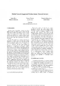
3.1.4. Load Balanced and Efficient Hierarchical Data-Centric Storage In [30] authors present a Hierarchical Voronoi Graph Based Routing (HVGR) algorithm. Taking the motivation from Voronoi graph, HVGR constructs and maintains a virtual hierarchy of sensor nodes. This hierarchical phenomenon is formed with self-organizing and without the help of any GPS or other geo-location devices. The network is divided into different levels of region based on landmarks. A landmark selection algorithm (discussed later) is used to select at most mi (i=1, 2, . . .) landmark in an (i-1)th level region. Then the network is first divided into first level sub regions based on first level landmarks. Each node in first level sub regions broadcast a landmark packet to the entire network. By receiving this packet every node estimates their distance from all first level sub-region landmarks. Each node selects one landmark as its representative. Then each first level sub-region is again divided into second level sub-regions with second level landmark. Each sensor node again chooses the closest landmark as their second representative. This process continues until the last level sub regions are small enough so that each node knows all other nodes in its sub region. D L1, 1, 1 3rd Level

L1

2nd Level L1, 1 S st

1 Level

Figure 5. Region Oriented Routing [30] 3.1.4.1. Routing Figure 5 shows an example of the basic routing algorithm which is used to route packets from the source (S) to the destination (D). The first level landmark of destination is L1. The packet first moves hop by hop toward L1 until it reaches the edge of first level region say R1. Now, nodes in R1 know the second level landmark and the packet now moves hop by hop toward second level landmark say L2. Again once it reaches the node B of Region 2 in Figure 5, the packet starts moving toward L3. Finally, the packet reaches the lowest level sub region whose entry node knows the path of destination and forwards the packet to the destination. The interesting part of this algorithm is it never overwhelms the landmark as the packets never go to the landmark rather they move toward the landmark until it reaches any node of that region. A series of hash functions Hi (i= 1, 2…) for each level of hierarchy is

introduced. H1 is used to enter into the first level region. Once the event enters the first level regions, H2 is used to enter second level region and so on. 3.1.4.2. Landmark Selection For landmark selection authors use optimized random landmark selection algorithm [36]. According to this algorithm, a random node, say A, starts the landmark selection process. A becomes the master landmark of first level landmark nodes. It selects m1-1 nodes for m1 first level networks. Each first level landmark then again acts as master and continues the selection process in its zone for selecting second level master node for second level of network. A master landmark node stops the landmark selection process once it finds that all sensor nodes in its region are within its communication range. 3.1.4.3. Load Balancing For balancing the load among sensor nodes, the basic name based routing is modified. During the landmark selection, the network is divided unevenly. For example, an event E has a probability 1/m1 of being assigned to the first level landmarks (L1, L2 . . .). If network is divided unevenly (L1>L2), L2 is more likely to be overloaded earlier than L1. Hence the load is balanced by assigning a task to regions in proportion to the sizes of the regions. An event is stored in a node in Lk’s first level region if and only if:

1 N

k −1

∑ N i ≤ H1 (E) ≤ i =1

1 N

k

∑N

i

i =1 m1

Here,

N i is the number of nodes in landmark Li’s first level region and N = ∑ N i i =1

3.1.4.4. Simulation and Evaluation The paper also discusses path stretch reduction and handling of dynamic changes. Proposed HVGR is simulated extensively and compared with Virtual Ring Routing (VRR) [37]. Using the result obtained from the simulation it is showed that HVGR outperforms VRR and achieves the goals: good scalability, good efficiency, and good load balancing for routing and data storage. 3.1.4.5. Discussion HVGR is proposed focusing mainly on the construction of virtual hierarchical relation among sensor nodes. It doesn’t consider range query, similarity search, data aggregation, non-uniformity and multireplication. Due to the lack of replication policy, HVGR is susceptible to data loss.

3.1.5. Dynamic Load Balancing Approach In [29], Wen-Hwa Liao et al. mention unbalanced distribution of data among sensors as one of the major constraint for most of the data-centric storage techniques. To address this issue, authors propose a grid-based dynamic load balancing (DLB) approach. DLB relies on two schemes: 1) a cover-up scheme to deal with a problem of a storage node whose memory space is depleted and 2) multithreshold levels to achieve load balancing in each grid and all nodes get load balancing. DLB divides the whole network in a grid with cells of the same size in such a way that all the nodes inside a cell are within one hop distance. Each grid is numbered with positive coordinates (X, Y) called grid IDs. A sensor node can calculate its grid ID (X, Y) using the following equation:

X = ( X i − X 0 ) / d  and Y = (Y1 − Y0 ) / d  Each node has a virtual grid ID and virtual co-ordinates which are initially equal to the actual grid ID and co-ordinates. Initially, each node broadcasts a message within its grid by limited broadcast to exchange the information of ‘Grid_Node’ table. A producer node uses the hash function on the event type which is mapped into a grid and transformed into a grid ID using above equation. The centre of the grid is called a grid point. The node, after detecting an event, sends a Put packet to the grid ID and uses a geographic routing protocol (GPSR) to forward this packet to node which is closed to the grid point.

3.1.5.1. Cover-up Scheme for Load Balancing To balance the load among sensors in a grid, a scheme named ‘cover-up’ scheme is used. According to this scheme every node of a grid has storage threshold levels. For instance, a sensor node has two levels of thresholds: 1st level = 30 and Second Level = 60. A grid point forwards and stores all packets in closest node of the grid. When the node closest to the grid point reaches first threshold level it modifies its virtual co-ordinate to (∞, ∞) in order to ‘cover-up’ its original location. Hence, the geographic routing protocol forwarding an event data to a storage node will ignore the original closest node and finds a new one which is next closest node to the grid point. This process continues until all nodes reach their first level of threshold. The last node, farthest from the centre, reaching this threshold notifies this fact and second threshold level of storage is established. However, following this mechanism at some point all the nodes within a grid could be saturated. In such case, the paper proposes extended grid, which is, using all the adjacent grids to the saturated one to select a new home node. When a query reaches a grid, all the sensor nodes of that grid receive this query and therefore, with the data stored in them, reply back to consumer. 3.1.5.2. Simulation and Evaluation The proposed model is simulated in Java assuming the hierarchy depth d=1. The total energy consumption simulated in this model includes energy consumption for both storing and retrieving an event. The energy consumption cost function is estimated based on the energy model [38]. The energy cost for sending a message S is determined by:

E send = Etrans * s + E amp * d 2 , where E trans is the

energy cost of sending a bit, S is the message size,

E amp is the energy consumed in the amplifier, and d

is the distance of message transmission. On the other hand, energy consumption for receiving a message is determined by a cost function: E send = E rec * r , where E rec is the energy cost of receiving a bit, and r is the message size. DLB is evaluated against GHT for total energy consumption, performance of the hot-spot storage space, the standard deviation of storage space, the average of storage space for load balancing, and finally the number of dropped events for the quality of data. 3.1.5.3. Discussion This proposal finds a smart way of changing home node in order to keep the load balanced. However, the paper doesn’t put focus on the recovery of data in the case of node failure and/or movement of a node from one zone to another. It also completely skips replication process which is very vital in the case of DCS. According to the core design of the paper, it can’t be scaled or extended for similarity search, data aggregation and range query.

3.1.6. Load Balanced Data-Centric Storage (LB-DCS) In [26], an organic approach named Load Balanced Data-Centric Storage (LB-DCS) scheme is proposed to overcome the constraint of load unbalance in DCS-GHT [1]. This is due to the fact that it relies on home perimeter for data replication. LB-DCS functions on top of three mechanism: i) A density estimation protocol. This protocol is used to estimate network density f which is included in put and get protocols; ii) A modified hashing function that includes f in its parameter list iii) a storage protocol enforcing QoS in the selection of number of replicas for data storage. In [39] authors claim that depending on the event type, the number of local replicas should be different. So, when a producer node produces any event it also specifies a value in terms of the parameter q to specify the number of replicas. The put primitive takes q along with two other parameters: datum d and meta-datum k. On the basis of this q parameter, home node selects q number of neighbour nodes using ball method to replicate that event. This dispersal method is iterative. The home node say H (with coordinates XH, YH) considers a ball with radius r (randomly selected value). It sends a request for storage to all sensors within the range of this ball denoted by:

B( X H ,YH ) (r ) = {sensors − of − coordinates ( x, y ) : ( x H , y H ), ( x, y ) < r} In turn, when a sensor receives storage request it acknowledges the request to H. H calculates the number of acknowledgment ( q ′ ) received from the nearest sensors. If q ′ < q , then H sends storage request

to

B( X H ,YH ) (2 ∗ r ) sensors.

This

time

it

considers

only

the

sensors

in

B( X H ,YH ) (2 ∗ r ) − B( X H ,YH ) (r ) . This process continues until H receives q number of acknowledgement or goes out of outermost perimeter. Apart from this quality of service, authors also include non-uniform hashing which can be used to balance the load even in non-uniform distribution say Gaussian distribution of sensor nodes in a network. For uniform hashing they have used Rejection Method [40]. 3.1.6.1. Network Density Estimation For handling dynamic network, the hash function includes network density estimation f. To the purpose of estimating sensor density, the WSN is divided into n x n non overlapping square regions of side p. The point at the centre is called watch point. A sensor node closest to watch point is called sentinel. After selecting the sentinel, each sentinel broadcasts a request to its neighbours to count them. The number of neighbours is used as an estimation of the local density in the region. One proactive protocol (Broadcast) and two reactive protocols (Stripes and FatStripes) are used to deliver the estimate computed by sentinels to other sensor nodes. In Broadcast, each sentinel sends its density information to all the sensors once during initial setup. In Stripes, density estimation is stored in every sensor along the unicast back route from sentinel. In turn, when a query for a sentinel arrives to a sensor it first checks its cache. If record is not found only then request is forwarded to the target sentinel. The FatStripes is the enhanced version of Stripes. As all the nodes in the transmission range spent same energy for receiving estimation of density, the estimation can be copied to all sensors who receive it. This obviously increases the probability of a hit during query. After collecting estimates a sensor uses

′

d i, j =

wij

∑

ij

wij

and

′

d ij =

′ m ∗ d ij + ∑

i ′ , j ′ ∈N ij

2∗m

d i′, j ′

′ for calculating density in each region and

final approximation based on first computation respectively. 3.1.6.2. Simulation and Evaluation For performance evaluation, both LB-DCS and DCS-GHT are simulated in the NS-2 simulator. The number of data stored in different nodes is measured for different load and it is shown that LB-DCS balances the load for both Uniform and Gaussian distribution. The number of MAC layer message exchange during get and put function is also measured for DCS-GHT and LB-DCS against different level of density. The graph presented in the paper [26] report, for different values of density, that LBDCS exchanges significantly lower number of MAC level messages than DCS-GHT. It also shows that put operation exchange more messages than get operation due to the dispersion mechanism inside the zone during get operation.

3.1.7. Tug-of-War In Tug-of-War [27], authors propose a data-centric mechanism where queries and events meet at a point selected based on the relative frequencies of events and queries. To minimize the communication cost, Tug-of-War adjusts the rendezvous point on the fly on an optimal basis. Tug-of-War takes motivation from Structured Replication (SR) mechanism in GHT. In SR, to alleviate node’s load, a detected event is stored in nearest mirror image. This mechanism alleviate storage cost but as query node has no idea which image node may have the data, it needs to query all the image, hence increasing query cost. However, this mechanism is useful if event detection frequency is much higher than event query frequency. Similarly, if query incurs more cost than events, then it is reduced by letting a node send its query message only to the nearest image, for this event need to be stored in all mirror images. 3.1.7.1. Modes of Operation ToW operates in two modes and they are referred as write-one-query-all and write-all-query-one. The former one allows a sensor to store an event in the nearest mirror image but queries need to be disseminated to all mirror images. Conversely, in the latter operation mode events must be stored to all mirror image to facilitate a query node to disseminate query only to nearest mirror image. In which mode a sensor node will operate depends on the resolution r. The resolution is determined based on the relative frequency of query and events detection for a particular class of event.

3.1.7.2. Routing Algorithm In ToW, authors also present a new routing algorithm namely: combing routing to replace hierarchical routing algorithm which is presented in SR-GHT to route a message to the set of all level-r images of an event class. Cost related to hierarchical routing in SR-GHT is shown by:

CR Hierarchical ≅ δ ( s, h) +

(2 + 2 ) n r (2 − 1) 2

≅ δ ( s, h) + [(1 + 2 ) ∗ 2 r − (1 + 2 )] n 2 2 Here,

CR Hierarchical = δ ( s, h) + S1 + S 2 + .......... + S r

δ ( s, h) = Distance between source node S and root image h Si = Distance between each (i-1) level image & associated three level i images. There are 4i-1 (i-1) level images and each (i-1) level image is associated with 3 i-level images. The cost of communication between each (i-1) level image to 3 associated i-level images is

n

2i

, n

2i

, 2

2i

∗ n. Hence,

S i = 4 i −1 ∗ ( =

2 2 + i ) n i 2 2

(2 + 2 ) n ∗ 2 i −1 2

On the other hand, in combing routing algorithm, cost consists of routing path from the message source

1 ) followed by 2 r vertical paths of the 2r same length. The distance d from the source to the nearest image is d = δ ( s, h) when r=0 and is δ ( s, h) halved for every increment of r. So, d = . So, total cost is defined by: 2r to the nearest image and a horizontal path of length

CRCombing ≅

δ ( s, h) 2

r

n (1 −

+ (2 r + 1)(1 −

1 ) n 2r

To optimize the sensor’s mode of operation based on resolution, it defines fe and fq referring event frequency and query frequency respectively. For, write-one-query-all the cost is defined by:

CW1Qall ≅ 2 2kδ Here,

fe fq

n

δ n = Average distance between a querying node and a home node of an event class K = Number of nodes detect events of a particular class denoted by C

Cost of write-one-query-all is defined by:

fq

CWall Q1 ≅ 2 2kδ

n

fe

3.1.7.3. Evaluation and Comparison ToW is analytically compared with another most close of this work referred to as Comb-Needle (CN) [41], where authors study push-pull event dissemination and query strategy in a grid network. Although CN and ToW both use dynamic strategy for information dissemination and gathering, there are some significant basic differences between them according to the author of ToW. Firstly, ToW is based on DCS while CN isn’t Data Centric, and so a query source in CN has no prior knowledge about which specific node to gather the information. As a result flooding is essentially a search technique. Secondly, through rigorous mathematical evaluation, it has been shown that ToW have smaller dominating constant in communication cost. As a result, on average the query latency of ToW is half of CN.

3.1.8. Similarity Search Algorithm Yu-Chi Chung et al. [21] propose similarity search algorithm (SSA) based on the concept of Hilbert Curve over a data-centric storage structure. SSA is successful in searching most similar data without collecting data from all the sensors in the network. Being motivated from the concept of Hilbert curve, authors divide the network recursively into 4l square quadrants where l denotes the number of levels. The centre (indexing node) of each square quadrant (cell) is denoted by I. It is important to select proper number of indexing node (I) to avoid performance degradation due to too many indexing node and on the other hand lack of enough storage space due to the fewer number of indexing nodes. If the total memory space for storing data is A and memory size of each sensor is z then the number of indexing node n can be defined as: n ≥  A Z  . So, the number of levels l is defined by:

l = log 4 n ≥  A z  . 3.1.8.1. Network Overlay The entire data range of an event is referred by R where RL and RU respectively denote lower bound and upper bound. R is divided into n equal sub-ranges each being equal to r i.e. n.r=R. So, the sub range of data for which IID is responsible is defined as

[R

I ID L

, RU

I ID

) = [R

L

+ ( I ID − 1) ⋅ r , RL + I ID ⋅ r ) .

Figure 6 illustrates for level 1 and level 2 assuming that the whole data range R of an event is (0, 1).

[0.25, 0.5) I1

[0.3125, 0.375) I5

[0.5, 0.75) I2

I4 [0.25, 0.3125) i=0.2

I0

I9

I10

I7

I11

I8 i=0.2

[0.125, 0.1875) I3 I2 [0.1875, 0.25)

I3 [0.75, 1]

[0, 0.25)

I6

I12

I13 I14

I0

I1 [0, 0.0625) [0.0625, 0.125)

I15 [0.9375, 1)

Figure 6. Level 1 and Level 2 Hilbert Curve [21] Any detected event mapped to a particular segment if the event fall in the range of that cell. Two parameters

ID

ID

(vmin , vmax ) are used to record the minimum and maximum existing values of each

segment. Initially these two parameters are set to 0. When a data is inserted in an index node, these two values are updated accordingly. For example, if a sensor detects an event with a value of 0.2 then the data is sent to I0 as it belongs to the range [0, 0.25) and both parameters will be update to

(vmin

ID

= 0.2, vmax

ID

= 0.2)

ID

ID

(vmin , vmax ) of this cell

3.1.8.2. Similarity Search When a data is queried it first forwards the query to the specific cell, range of this cell contains the queried data, and then try to find the closest value. The presented similarity search mechanism contains two phases, the similarity search query resolving phase and the query probing phase. The query resolving phase determines an indexing node that is most likely to provide an answer for the query. If the answer doesn’t match exactly then the query probing phase is initiated for finding possible closest answer. In Query Resolving Phase, the following locate() function is used to find the Target Node IT. locate (Vq) = locate the indexing node IID such that RL + ( I ID − 1).r ≤ Vq < RL + I ID .r , where Vq is the search value given by the query. The query is then forwarded to the Target Node IT to retrieve data. If an exact match to Vq is found then the query execution is finished otherwise query probing phase comes in action. In query probing phase there can be two following possible cases: • Case 1: IT is non-empty and o

Sub-case 1: If

I

vs T is the most similar local data in IT.

I

vs T is larger than vq , then all data in IT+1 must be even greater than vq . But

in IT-1 there may be a vs o

Sub-case 2: If to vq than

IT −1

which is closer to vq .

IT

vs is smaller than vq , then all data in IT-1 must not be more similar

I

vs T is. But in IT+1 there may be a vs

• Case 2: IT is empty (i.e. no data stored).

IT +1

which is closer to vq .

vq has to be sent to both neighbours (i.e. IT-1 and IT+1) of IT

to find the most similar data. Three functions are proposed referred as: backward probing, forward probing and bi-directional probing. Backward probing and forward probing are used to deal with Case 1 while bi-directional probing is used to for Case 2. 3.1.8.3. Index Node Handoff and Failure Two methods are proposed for workload sharing. One case is when an indexing node fails due to power shortage. In this case, once the power level of a sensor goes beyond certain threshold, can be system defined or pre-installed, other sensor takes the responsibility. The basic idea is to transfer the current jobs and the data to a nearby sensor. In the second case a node fails due to sudden unexpected damage. In this scenario, data has to be duplicated in the mirror indexing node. Neighbours of this victim indexing node are aware of this failure, so when a detected data/query is sent to this failed indexing node through these neighbours, they will locate the mirrored indexing node by using the mirror mapping function and forward the data to that new indexing node. 3.1.8.4. Range Query Authors also extend their work into range query processing for both single and multi-dimensional attributed. A range query is divided into sub-queries and then the sub-queries are forwarded to their corresponding indexing node. For example, the level of carbon monoxide of air in a forest, the number of level of the network 1, ranges from 50 L/mol to 150 L/mol. Then this range is split equally into four (41=4, four index node referred as I0, I1, I2, I3) sub ranges [50, 75), [75, 100), [100, 125), [125, 150). Hence, if a range query is to find data within [60, 80], then the sub-ranges of I0 and I1 are located as they cover the given query. 3.1.8.5. Simulation and Evaluation The model SSA is simulated and evaluated against SR-GHT and naïve algorithm for network size, node density, node distribution and the number of levels of a Hilbert curbe. As communication cost is the main part of energy consumption, hence number of exchanged messages is used as the comparison metrics for evaluation.

3.2. Data Centric Conveyance based on Tree-Structures 3.2.1. A Distributed Index for Features in Sensor Network A Distributed Index for Features (DIFS) in Sensor Network [20] is designed to provide balance on communication load across the index keeping the search efficiency of a quad tree [42]. DIFS also uses Geographic Hash like GHT [1]. DIFS constructs a multiply rooted hierarchical index that differs from traditional binary and quaternary trees. In DIFS a non-root tree can have multiple parents. Nodes are responsible for storing information for a specific range within a particular geographic region. A node covering small area stores wider range of values while a node covering large area stores small range of values. DIFS efficiently supports range queries, queries related to distribution of values in space and so forth. DIFS constructs a search hierarchy of histograms, but unlike single tree hierarchies of structured replication and quad tree, each child in DIFS has bfact (bfact= 2i where i > 1) parents. The range of values a child maintains in its histogram is bfact times the range of values maintained by its parents. The range of values that an index node knows about is inversely related to the spatial extent the node covers. This helps to ensure a balance of communication load over the network. A search in DIFS may originate from any node of the tree. A node, storing an event, forwards information first to the local index node with the narrowest spatial coverage but covering the widest value range. A histogram describing the values is then forwarded to a node with wider spatial coverage but narrower value range from current index node. This process keeps on going and so on and so forth. Unlike GHT, DIFS function takes string of characters, source location and a bounding box to hash function producing a hash location. 3.2.1.1. Simulation and Evaluation In simulation and analysis, authors take Quad tree, Diffusion and Structured Replication using numerical simulations to compare with DIFS. Based on the simulation result provided by authors, structured replication [1] outperforms DIFS and Quad tree [42] approach in terms of communication for storage. The reason given is that the initial registration of event with Structured Replication’s (SR) local leaf level mirror point needs no additional work. However, queries with sufficiently constraint search criteria DIFS and Quad Tree lead to the pruning of branches in the search tree consequently generating lower search costs than SR. On the other hand, in the case of queries requesting most of the entire range data results in no pruning, DIFS and Quad tree don’t perform better than SR. However, average bottleneck utilization is significantly reduced when the query range is sufficiently constrained. In quad tree, like DIFS, the bottleneck is always the root and its utilization is 1 while in SR every node of the tree is explored during every search. In terms of aggregate communication cost of storage and of search quad tree outperforms DIFS but it is not scalable to a large number of searches or stores. Using multiply rooted tree and a trade-off between geography/value coverage DIFS scales well to a large extent.

3.2.2. Practical Data-Centric Storage In PathDCS [43], few shared points of reference named landmarks are used and name locations by their path from one of these shared points of reference. PathDCS define tree-structures in order to route messages. The interesting novelty of this approach is that an event type is mapped to a path instead of mapping it to a spatial location. The path is defined by an initial landmark and then followed by a set of procedural directions. The landmarks are also called beacon nodes which are elected randomly or manually configured. Standard tree construction techniques are use used to build trees rooted at each of these beacon nodes. This ensures all nodes know how to reach beacons. A path consists of a sequence of p beacons bi and length li where i=1, 2 … p. The packet is first routed to beacon b1, and then it is sent l2 hops toward beacon b2 using the tree rooted at b2, and so on, until it is ended up at the previous i-1 segment, it is then sent li hops toward the next beacon bi. A beacon node bi is the beacon whose identifier is closest to the hash function h (k, i). In addition, the first segment length l1 is equal to the distance to the first beacon b1, whereas segment lengths for i > 1 are given by:

l i = h(k , i ) mod hops (ni , bi ) pathDCS algorithm has two parameters: the total number of beacon nodes denoted by B and the number of path segments referred as P. The performance of pathDCS largely depends on these two

parameters. Minimisation of beacon nodes helps to minimise overhead. Data is also been locally replicated by flooding within k-hops of the destination. 3.2.2.1. Beacon Handoff and failure Role of beacons are handed over to other nodes periodically. This happens to avoid node failure or to reduce the forwarding load on previously selected beacon nodes. Every beacon nodes maintain a threshold value measuring link quality. If the link quality goes under threshold value all single hop nodes participate in beacon selection process. The winning node in the beacon selection process decease the current beacon node and assumes that role henceforth. For the latter case, deliberate handoff, beacon randomly selects a neighbour node and exchanges its identifier with it. 3.2.2.2. Simulation and Evaluation Performance evaluation is done through both high-level and packet-level simulations, as well as through experiments on a sensor node test bed. The simulation is conducted over TOSSIM. Authors correlate percentage of total transmission (increases exponentially) with the percentage of nodes. Success probability is also tested under failure and randomized parent selection for increasing network sizes. PathDCS is also implemented in TinyOS and evaluated on the 100-node Intel Mirage micaZ testbed as well as on 500 nodes in TOSSIM packet-level emulator. 3.2.2.3. Discussion DCS methods have been classified into generations in this paper namely point-to-point and treestructures. Authors preferred later one pointing out different problems about former routing method. PathDCS mainly focuses on tree construction, and hence query mechanism left out of focus. However, authors also totally ignore other major challenges like range query, similarity search, data aggregation, load balance and dealing with non-uniformity.

4. Conclusion Over the past two decades a large amount of research work has been done on wireless sensor network. However, the history of Data Centric Storage is less than one decade. Since sensor network is becoming a prime source of data collection, DCS is of pivotal importance. The key DCS mechanisms have been classified in this chapter and are summarized in Table 2 for convenience. It is clear that with the passage of time, researchers are addressing new challenges relevant to DCS and trying to provide solution as well. However, from the Table 2 it is apparent that very few works put focus on few recently investigated but important challenges such as similarity search, spatial-temporal search, dynamic load balance, data aggregation and dealing with non-uniformity. The emerging new researchers can take this chapter as a very potential source of state-of-art about previous and current research in DCS and push their knowledge and invention toward the enrichment of this field accordingly. Table 2. Comparison of DCS Methods Title

1

2

3

4

Geographic Hash Table (GHT) [1] Data Storage and Range Query Mechanism for Multi-dimensional Attributes. [18] Distributed SpatialTemporal Data Storage Scheme. [19] Load Balanced and Efficient Hierarchical Data-Centric Storage. [30]

5

Dynamic Load Balancing Approach [29]

6

Load Balanced Data-

Routing Category

Dimension (attribute)

Range vs. Point Query

Data Aggregation

Similarity Search

Multi Replication

Load Balance

Point-toPoint Routing

Single

Point

No

No

No

No

Point-toPoint Routing

Multi

Range

No

No

No

No

Point-toPoint Routing

Multi

Range

No

Yes

No

Yes

Point-toPoint Routing

Single

Point

No

No

No

Yes

Single

Point

No

No

No

Yes

Single

Point

No

No

No

Yes

Point-toPoint Routing Point-to-

Centric Storage (LBDCS) [26] 7

Tug-of-War [27]

8

Efficient Mechanism for Similarity Search [21]

9

DIFS: A Distributed Index for Features in Sensor Network [20]

10

PathDCS [43]

Point Routing Point-toPoint Routing Point-toPoint Routing DCS Based on TreeStructure DCS Based on TreeStructure

Single

Point

No

No

Yes

No

Both

Both

No

Yes

No

Yes

Single

Range

No

No

No

No

Single

Point

No

No

No

No

5. Bibliography [1] [2] [3] [4] [5] [6] [7] [8] [9] [10] [11] [12] [13] [14] [15] [16] [17] [18]

S. Ratnasamy, et al., "GHT: a geographic hash table for data-centric storage," presented at the Proceedings of the 1st ACM international workshop on Wireless sensor networks and applications, Atlanta, Georgia, USA, 2002. G. Campobello, et al., "A novel reliable and energy-saving forwarding technique for wireless sensor networks," 2009, pp. 269-278. G. J. Pottie and W. J. Kaiser, "Wireless integrated network sensors," Communications of the ACM, vol. 43, pp. 51-58, 2000. S. Saroiu, et al., "A measurement study of peer-to-peer file sharing systems," 2002, p. 152. Y. Yao, et al., "In-network processing of nearest neighbor queries for wireless sensor networks," 2006, pp. 35-49. R. Szewczyk, et al., "Lessons from a sensor network expedition," Wireless Sensor Networks, pp. 307-322, 2004. C. Intanagonwiwat, et al., "Directed diffusion: a scalable and robust communication paradigm for sensor networks," presented at the Proceedings of the 6th annual international conference on Mobile computing and networking, Boston, Massachusetts, United States, 2000. W. Zhang, et al., "Data dissemination with ring-based index for wireless sensor networks," 2003, pp. 305-314. S. Madden, et al., "TAG: a Tiny AGgregation service for ad-hoc sensor networks," SIGOPS Oper. Syst. Rev., vol. 36, pp. 131-146, 2002. F. Ye, et al., "Gradient broadcast: A robust data delivery protocol for large scale sensor networks," Wireless Networks, vol. 11, pp. 285-298, 2005. F. Ye, et al., "A two-tier data dissemination model for large-scale wireless sensor networks," 2002, pp. 148-159. S. Ratnasamy, et al., "Data-centric storage in sensornets with GHT, a geographic hash table," Mobile networks and applications, vol. 8, pp. 427-442, 2003. X. Li, et al., "Multi-dimensional range queries in sensor networks," presented at the Proceedings of the 1st international conference on Embedded networked sensor systems, Los Angeles, California, USA, 2003. D. Ganesan, et al., "DIMENSIONS: Why do we need a new Data Handling architecture for Sensor Networks?," ACM SIGCOMM Computer Communication Review, vol. 33, pp. 143148, 2003. D. Ganesan, et al., "Networking issues in wireless sensor networks," Journal of Parallel and Distributed Computing, vol. 64, pp. 799-814, 2004. I. Chatzigiannakis, et al., "An adaptive power conservation scheme for heterogeneous wireless sensor networks with node redeployment," 2005, pp. 96-105. K. P. Shih, et al., "CollECT: Collaborative event detection and tracking in wireless heterogeneous sensor networks," Computer Communications, vol. 31, pp. 3124-3136, 2008. W. H. Liao and C. C. Chen, "Data storage and range query mechanism for multi-dimensional attributes in wireless sensor networks," Communications, IET, vol. 4, pp. 1799-1808, 2010.

[19] [20] [21] [22] [23] [24] [25] [26] [27] [28] [29] [30] [31] [32] [33] [34] [35] [36] [37] [38] [39] [40] [41] [42] [43]

H. Shen, et al., "A Distributed Spatial-Temporal Similarity Data Storage Scheme in Wireless Sensor Networks," Mobile Computing, IEEE Transactions on, vol. 10, pp. 982-996, 2011. B. Greenstein, et al., "DIFS: a distributed index for features in sensor networks," in Sensor Network Protocols and Applications, 2003. Proceedings of the First IEEE. 2003 IEEE International Workshop on, 2003, pp. 163-173. Y.-C. Chung, et al., "An efficient mechanism for processing similarity search queries in sensor networks," Information Sciences, vol. 181, pp. 284-307, 2011. A. Ghose, et al., "Resilient Data-Centric Storage in Wireless Ad-Hoc Sensor Networks," presented at the Proceedings of the 4th International Conference on Mobile Data Management, 2003. S. R. Madden, et al., "TinyDB: an acquisitional query processing system for sensor networks," ACM Transactions on Database Systems (TODS), vol. 30, pp. 122-173, 2005. G. Amato, et al., "MaD-WiSe: programming and accessing data in a wireless sensor networks," 2005, pp. 1846-1849. A. Cuevas, et al., "Modelling data-aggregation in multi-replication data centric storage systems for wireless sensor and actor networks," Communications, IET, vol. 5, pp. 1669-1681, 2011. M. Albano, et al., "Dealing with Nonuniformity in Data Centric Storage for Wireless Sensor Networks," Parallel and Distributed Systems, IEEE Transactions on, vol. 22, pp. 1398-1406, 2011. Y.-J. Joung and S.-H. Huang, "Tug-of-War: An Adaptive and Cost-Optimal Data Storage and Query Mechanism in Wireless Sensor Networks." vol. 5067, S. Nikoletseas, et al., Eds., ed: Springer Berlin / Heidelberg, 2008, pp. 237-251. Á. C. Rumín, et al., "Data Centric Storage Technologies: Analysis and Enhancement," Sensors, vol. 10, pp. 3023-3056, 2010. W.-H. Liao, et al., "A grid-based dynamic load balancing approach for data-centric storage in wireless sensor networks," Computers & Electrical Engineering, vol. 36, pp. 19-30, 2010. Z. Yao, et al., "Load Balanced and Efficient Hierarchical Data-Centric Storage in Sensor Networks," in Sensor, Mesh and Ad Hoc Communications and Networks, 2008. SECON '08. 5th Annual IEEE Communications Society Conference on, 2008, pp. 560-568. I. Stoica, et al., "Chord: A scalable peer-to-peer lookup service for internet applications," SIGCOMM Comput. Commun. Rev., vol. 31, pp. 149-160, 2001. P. Maymounkov and D. Mazieres, "Kademlia: A peer-to-peer information system based on the xor metric," Peer-to-Peer Systems, pp. 53-65, 2002. A. Rowstron and P. Druschel, "Pastry: Scalable, decentralized object location, and routing for large-scale peer-to-peer systems," 2001, pp. 329-350. B. Karp and H. T. Kung, "GPSR: greedy perimeter stateless routing for wireless networks," 2000, pp. 243-254. G. G. Finn, "Routing and addressing problems in large metropolitan-scale internetworks," DTIC Document1987. Y. Zhao, et al., "Efficient hop id based routing for sparse ad hoc networks," 2005, pp. 10 pp.190. M. Caesar, et al., "Virtual ring routing: network routing inspired by DHTs," ACM SIGCOMM Computer Communication Review, vol. 36, pp. 351-362, 2006. W. R. Heinzelman, et al., "Energy-efficient communication protocol for wireless microsensor networks," 2002, p. 10 pp. vol. 2. M. Albano, et al., "Q-NiGHT: Adding QoS to Data Centric Storage in Non-Uniform Sensor Networks," in Mobile Data Management, 2007 International Conference on, 2007, pp. 166173. J. Von Neumann, "Various techniques used in connection with random digits," Applied Math Series, vol. 12, p. 1, 1951. X. Liu, et al., "Combs, needles, haystacks: balancing push and pull for discovery in largescale sensor networks," 2004, pp. 122-133. R. A. Finkel and J. L. Bentley, "Quad trees a data structure for retrieval on composite keys," Acta informatica, vol. 4, pp. 1-9, 1974. C. T. Ee and S. Ratnasamy, "Practical Data-Centric Storage," in Conf. Networked Systems Design and Implementation (NSDI'06), 2006.