Data Coordination: Supporting Contingent Updates Michael Lawrence
Rachel Pottinger
Sheryl Staub-French
Dept. of Computer Science University of British Columbia Vancouver, Canada
Dept. of Computer Science University of British Columbia Vancouver, Canada
Dept. of Civil Engineering University of British Columbia Vancouver, Canada
[email protected]
[email protected]
[email protected]
ABSTRACT
to this problem of updating an existing data source based on changes in independently maintained data sources as data coordination. Other data coordination scenarios arise; for example, a bus company may need route data to coordinate with the road network data provided by the city, a national department of finance may need to coordinate economic indicators with data provided by local statistics gathering bodies, or a ferry operator may need to coordinate its schedule information based on data from a marine forecast website. More specifically, data coordination occurs between two autonomous but related data sources, B and C. In particular, one provider (e.g. the building architect) maintains a base relational database, B, while another provider (e.g. the contractor) maintains its own, separate, contingent relational database, C. This is in contrast to the traditional problem of data integration [6], which focuses on querying heterogeneous data; and coordination in peer to peer databases [10, 13, 16], where a number of participants use a common system to share data. We address coordination scenarios where there is a lack of system wide collaboration: C is interested in coordinating with data made available by an autonomous source B, with B periodically changing without notice due to external factors (e.g. the architect updates the design due to client requests). Our proposal for data coordination is a system which can be used by the administrator of C to detect relevant changes in B and compute a set of updates to C in order to maintain consistency. This presents the following new challenges from previous work on data coordination [2, 9, 16] for several reasons: 1) the loose coupling of B and C means that C will not receive notifications when and how B has changed; 2) the base/contingent relationship constrains coordination to only modifications on C, and 3) the contingent source C is interested in resolving a final ground instance and must be careful to avoid changes which result in other side-effects. In this paper, we propose a data coordination system which represents relationships between B and C using declarative mapping constraints of the form qB = qC .1 Such constraints permit the straightforward expression of complex relationships between sources. Our system monitors B for changes which impact C and performs best-effort coordination using a two-phased approach: 1) View Differencing, which finds the changes to the view defined by qB = qC , and 2) Update Translation, which translates these into changes to C, allowing its administrator to review and select the
In many scenarios, a contingent data source may benefit by coordinating with external heterogeneous sources upon which it depends. The administrator of this contingent source needs to update it when changes are made to the external base sources. For example, when a building design is updated, the contractor’s cost estimate must be updated, too. The goal of data coordination is to update a contingent source, C, based on changes to an independently maintained base source, B. This paper introduces a data coordination system which allows C to coordinate its data without imposing significant requirements on B. Our system uses declarative mappings between B and C and performs coordination in two stages View Differencing — finding changes to an intermediate view of B based on its mapping to C, and Update Translation — translating the view differencing result into updates on C. We present and evaluate novel solutions to both stages and demonstrate their feasibility on real world problems.
1.
INTRODUCTION
In many applications, a data source may need to be coordinated with heterogeneous data sources on which it depends. The administrator of this contingent source needs to ensure it is up to date and consistent with the latest data provided by these base sources. A significant challenge when coordinating between autonomous sources is that the base sources only participate in the process to the extent of providing access to their data: the entire coordination process is the responsibility of the contingent source’s administrator. For example, a precise cost estimate is critical for decision making during a building’s design phase. Updated building designs are periodically provided by the project’s architect, while the cost estimate is created and maintained by the contractor. Efficiently determining how the building design changes and what effects these changes have on the cost estimate are significant challenges for the contractor. We refer Permission to make digital or hard copies of all or part of this work for personal or classroom use is granted without fee provided that copies are not made or distributed for profit or commercial advantage and that copies bear this notice and the full citation on the first page. To copy otherwise, to republish, to post on servers or to redistribute to lists, requires prior specific permission and/or a fee. Articles from this volume were invited to present their results at The 37th International Conference on Very Large Data Bases, August 29th - September 3rd 2011, Seattle, Washington. Proceedings of the VLDB Endowment, Vol. 4, No. 11 Copyright 2011 VLDB Endowment 2150-8097/11/08... $ 10.00.
1 A much altered definition of data coordination appears in [18], which takes a substantially different approach.
831
id 0 1 2 cid 0 0 1 1 2
type length height Column 1 1 Wall 10 3 Wall 4 3 (a) Component
area 1 27 12
name/desc light concrete heavy concrete drywall
Figure 3: VB , the evaluation of qB on building design Bt (Figure 1) equals VC , the evaluation of qc on cost estimate Ct (Figure 2).
name thickness column concrete 240 rebar 200 light concrete 300 drywall 15 heavy concrete 200 (b) Material
Building Architect
code qty 2220.00 1 3100.04 30 9250.12 27 9250.14 12 9250.02 27 (a) ProjectItems
desc column formwork column rebar light concrete heavy concrete drywall 190mm studs (b) ItemRates
Contractor
V
diff?
Cost Estimate (C)
rate 6.50 165.00 25.00 35.00 3.50 12.00
Figure 4: The Cost Estimator stores view V on the building design. When V changes, we translate these changes into a set of changes on C.
declarative mapping constraint qB = qC defined by the following queries VB (nm, ar) :− Component(id, t, l, h, ar) ∧ Material(id, nm, th)
Figure 2: Example cost estimate Ct .
VC (desc, qty) :− ProjectItems(c, qty) ∧ ItemRates(c, desc, r) ∧ c = 9250.∗
suggested changes. We make the following specific contributions: • We define data coordination and decompose the problem into view differencing and update translation.
expressing the relationship between the walls in the building design and the cost items pertaining to walls in the cost estimate. The data of Figures 1 and 2 satisfy this mapping because evaluating qB on Bt yields the same result as evaluating qC on Ct (Figure 3). 2
• We propose and experimentally evaluate two algorithms for view differencing. • We propose algorithms for view update translation based on data exchange formalisms [7] and incomplete information [8] which find all possible translations, and guide the user to select a unique solution.
Our data coordination system would allow the Cost Estimator to coordinate C with building design B. The Cost Estimator describes how to connect to B and the desired mapping to be maintained. Our system uses a “pull” model of coordination, which is appropriate for scenarios where B is unwilling to make special provisions to support coordination of contingent sources (for example if B is a dataset available through a public URL). Our system stores a materialized view V on the building design as defined by the query qB . It monitors B, and when there are changes to V, it computes a set of possible changes to C as shown in Figure 4. A major challenge is handling ambiguity. In Example 1 if the building architect removes the drywall material layer from Wall 1, it will cause (drywall, 27) to be deleted from V, which could be reflected in the cost estimate by deleting from ProjectItems, ItemRates, or both. A more challenging example is if the building architect adds paint layers to Walls 1 and 2, causing (beige paint, 88) to be inserted into V. This will require inserting into both ProjectItems and ItemRates, but we cannot tell which value to use for its rate or code (although qC tells us c = 9250.∗). If there is an existing “beige paint” tuple in ItemRates, then there is a good chance that we can use its code and insert a single tuple into ProjectItems. However, real world construction data is ambiguous, containing duplicate descriptions and codes.
• We experimentally evaluate our update translation algorithms on real-world data, demonstrating their feasibility and the benefit of practical heuristics. The remainder of this section presents an example which outlines our data coordination approach. Section 2 introduces our data coordination system and formally defines the specific problems we address. Section 3 outlines and presents experimental results for two approaches to view differencing; Section 4 describes our solutions for update translation, followed by experimental results in Section 5, related work in Section 6, and conclusions in Section 7.
1.1
Building Design (B)
qB
Figure 1: Example building design Bt . code 3100.04 3100.08 9250.12 9250.14 9250.02 9250.03
ar/qty 27 12 27
Motivating Example
Example 1. A Building Designer’s data has schema B containing relations Component and Material. An instance Bt at time t is shown in Figure 1. A Cost Estimator’s data has schema C containing relations ProjectItems and ItemRates; they have created an instance Ct in Figure 2 for the building design Bt . The Cost Estimator has also created a
832
Bt+1
Because of these ambiguities, both examples remain nontrivial even if Bt were given. Our approach to data coordination is to provide a concise description of all possible solutions, given the changes and mapping constraint. This approach is motivated by the user’s need to resolve a final ground instance of C. It allows them to retain control over how coordination is performed, and provides opportunities to overlay situation-dependent ranking strategies.
2.
qB
Vt qC
Ct
(V+, V-) (C+, C-)
Vt+1 Ct+1
Figure 5: Data coordination solution overview.
DATA COORDINATION
every day or every week. The central problem addressed by our system occurs each time a change is detected in B:
Our system uses declarative mapping constraints of the form qB = qC to express the coordination relationship of B to C. As emphasized in [15], using declarative mappings allows the mapping designer to focus on what it means to be coordinated, without concern to how coordination is achieved. In this section, we formally define the specific problems addressed in the implementation of our coordination system. A database schema A is a set of relations, {A1 , . . . Ak }, and an instance A of schema A consists of a set of relation instances {A1 , . . . Ak }. A query q over A is a function from instances of A to instances of a view schema, which we denote V , writing the query as V (x) :− q(x, y), where x is the set of attributes of V , q is a conjunction of relational predicates, and y is the set of attributes in these relational predicates which are not in x. In query qB of Example 1, x consists of nm, ar, while y consists of id, t, l, h, th. When it is clear from the context, we also use V = q(A) to denote the set of tuples which results from evaluating q on A. Our mappings are defined as follows.
Definition 3. (Data Coordination Problem) Given 1. Schema B, database instance Bt+1 2. Schema C, database instance Ct 3. A mapping constraint qB = qC s.t. there exists some Bt s.t. qB (Bt ) = qC (Ct ) Find all possible updates (C+ , C− ) such that when applied to Ct , the result is a Ct+1 such that mapping qB (Bt+1 ) = qC (Ct+1 ) is satisfied. 2
2.1
Our Approach
In our approach to data coordination, the mapping qB = qC captures the subset of B’s data which, were it to change, should have an effect on C. We can thus focus our data coordination efforts by examining only what has changed with respect to the view defined by qB . As discussed above, our system implements coordination by storing a materialized view V on B defined by qB . C is coordinated with B when V is identical to the materialized view VC resulting from applying qC to C. Hence, if V is unavailable, it can be recomputed from C. With respect to the data coordination problem defined above, at time t + 1, C will have a materialized view Vt on B at the time t when it was last coordinated, thus providing a record of the exact changes to B which are pertinent to C. We use Vt to break data coordination into the following two stages:
Definition 1. (Mapping Constraint). A mapping constraint between relational schemas B and C is an expression of the form qB = qC , where qB is a query over B, qC is a query over C, and both qB and qC have the same number and types of attributes in x. A mapping constraint qB = qC is said to be satisfied with respect to instances B and C if qB (B) = qC (C). 2 Our approach in general is for conjunctive queries qB and qC , although we note that one of the proposed methods permits arbitrary queries for qB , and that extending to queries with arithmetic comparisons is a topic of our ongoing work. The problem of creating mappings is outside the scope of this paper. It has recently been argued [5] that precisely engineered mappings are needed in many applications, and we leave this responsibility to a domain expert (e.g. the Cost Estimator), who may draw assistance from automated tools such as Clio [20]. Data coordination involves updating the contingent source, C, in response to changes in the base source, B. We define an update as follows:
1. (View Differencing) Given Vt and Bt+1 , find updates (V+ , V− ) to Vt s.t. qB (Bt+1 ) = (Vt ∪ V+ ) − V− . + − + − 2. (Update Translation) ` Given (V , V´ ), find (C , C ) s.t. qB (Bt+1 ) = qC (Ct ∪ C+ ) − C−
This approach is illustrated in Figure 5. In Section 3 we propose two methods to view differencing: 1) a practical and straightforward method which finds (V+ , V− ) by materializing Vt+1 and comparing it with Vt ; and 2) an approach which is adapted from incremental view maintenance. We experimentally investigate important questions about the behavior and performance of these methods. Update translation is the more challenging stage and represents the bulk of this paper. The challenge with update translation is ambiguity: there may be many possible translations of (C+ , C− ) for a given (V+ , V− ). This challenge is compounded by the need for exact equality: how do we find a translation which avoids side-effects? (spurious insertions or deletions.)
Definition 2. (Update) An update to an instance A is − a set of pairs of tuple sets (A+ i , Ai ) for each relation Ai . The result of applying an update (A+ , A− ) to A is {(A1 ∪ − + − A+ 1 ) − A1 , . . . (Ak ∪ Ak ) − Ak } We assume that for all i + − A− ⊆ A and A ∩ A = ∅. 2 i i i i Since B is autonomous and does not push change notification to C, our system must monitor B for changes. The monitoring policy depends on the freshness requirements of Cs administrator — for example, our system might check B
833
The problem is related to data exchange [7]; however, data exchange uses open world semantics and considers the generation of a target source from scratch (as opposed to updating an existing source.) Hence their constraints are more relaxed than in data coordination: the view need only be a subset of a given query on a database instance. Our approach is to translate insertions and deletions separately. We combine methods from data exchange, and use incomplete information to define a universal solution for insertion translation which avoids side-effects (Section 4.1). We then formally define the set of minimal, feasible deletion translations and propose a constrained search method which finds them (Section 4.2). In Appendix C, we discuss how these translations are combined into the final result in our system, as well as a number of practical enhancements.
3.
our solutions to its implementation challenges for data coordination are given in Appendix A. The following section describes the results of experimentally comparing MAC to IVM-VD. While the heuristic of inertia [11] states that IVM-VD should be preferred for small updates, there are a number of practical reasons to prefer MAC. We consider the exploration of such trade-offs an important contribution; to our knowledge, there has been no prior comparison of the performance benefits of incremental view maintenance as opposed to materializing from scratch.
3.3
VIEW DIFFERENCING
3.1
Materialize and Compare
Our first proposed approach to view differencing is to materialize Vt+1 by evaluating qB on Bt+1 , and generate (V+ , V− ) by direct comparison with Vt . We call this Materialize and Compare (MAC). We briefly describe MAC here; details are in Appendix A. MAC computes (V+ , V− ) by scanning Vt and Vt+1 in parallel. The process is similar to a sorted merge: the next tuples from each of Vt and Vt+1 are compared via a total ordering; if one is smaller than the other, it is added to V− or V+ (if it came from Vt or Vt+1 respectively). MAC for view differencing has several benefits:
1. Both MAC and IVM-VD are feasible, offering acceptable performance under realistic conditions. 2. IVM-VD’s execution time varies exponentially with the number of joined relations in qB , but only if most of these relations are updated. MAC is fairly resilient to changes in the problem parameters; its performance depends mostly on the size of Vt and Vt+1 . Both algorithms are linear in the size of the instance.
1. Since we are simply evaluating qB , there is no limit to the types of queries which can be used. This allows for mappings expressing very sophisticated relationships, e.g. aggregation, conditionals, negation etc.
3. MAC appears to be favorable to IVM-VD when qB contains more than a few joins, and the size of the updates is greater than 2.5% of the database instance.
2. Minimal support is required from source B. As stated in Section 1, one goal is to support autonomous sources. For the MAC algorithm, we only require B to evaluate queries on the its current data instance.
3.2
Comparing MAC to IVM-VD
IVM-VD should be more efficient than MAC when the updates are small and recomputing the view from scratch is expensive. However, there are several possibly limiting factors: IVM-VD makes a trade-off between the number of queries evaluated, and the cost of each of these evaluations. The reasoning is that it should be more efficient to evaluate a large number of delta rules, each involving a term (B+ i or B− ) significantly smaller than the base relations. Of course, i the performance advantage gained by this trade-off depends on the number of relations in the query qB and the number of inserted/deleted tuples for each of these relations. We explore the scope of this trade-off in depth in Appendix A.1; our findings are as follows:
4.
UPDATE TRANSLATION
After our system has computed a set of updates (V+ , V− ) to V, it attempts to translate these into a set of updates on C. A satisfactory translation requires that evaluating the query qC on the updated C results in the updated view. The problem is extremely challenging because, as shown in [3], unambiguous translation is only possible under extremely limited conditions. Update translation for data coordination additionally poses some new challenges for the following reasons:
Incremental View Maintenance
Our second approach to view differencing is based on an adaption of incremental view maintenance (IVM) techniques, hence we call it IVM for View Differencing (IVMVD). IVM [11] updates a materialized view given changes to the base relations without recomputing that view from scratch. IVM, in addition to the new base relations (Bt+1 ) and existing materialized view (Vt ), also requires access to the old base relations (i.e. Bt ) and the updates to the base relations. Its result is Vt+1 . We use the counting algorithm of [12], which requires a count of the distinct derivations of tuples in the view. Briefly, for a query with k predicates, the counting algorithm evaluates the additive union of 2k separate query evaluations (delta rules), each replacing one of the relational predicates with its updates. Implementing this algorithm within the context of an autonomous data coordination system requires two major changes: 1) A local query rewriting to obtain tuple counts from B without requiring any special facilities; and 2) a modified implementation of the additive union operator which allows the view updates to be isolated during the computation of Vt+1 . The full IVM-VD algorithm and
1. Our solution must be exact. That is, our mapping constraints demand equality (bi-directional logical implications), as opposed the more common subset constraints (uni-directional implication.) This means that special attention must be paid to side-effects; we need to ensure translated insertions C do not cause additional, spurious insertions into VC 2. Because changes to C are dictated by the given changes to V (which are dictated by changes to B), updates to C must not assert additional changes to V. 3. We need to consider sets of insertions and deletions, and the interaction between them. I.e. translating each
834
4.1.1
insertion or deletion separately and taking the union will produce incorrect results.
The chase step translates the set of insertions by chasing [4, 7] to find a universal solution to the data exchange problem given V+ and the constraint from Equation (1) in Section 4.1. The correctness of our approach relies on the following theorem.
+
Our methods for translation of insertions V make use of the tuple generating dependency (tgd) chase [1]. In doing so, we generate an uncertain translation containing free variables. A similar approach in a peer to peer setting is taken in Youtopia [9, 16], where individual insertions and deletions are propagated amongst a peer data sharing network. We then find constraints on these variables by using algebra of incomplete information [8]. This translation is presented to the administrator of C, who should have some domain knowledge which allows them to fill in the missing values.
4.1
Chase Step
+ Theorem 1. Let {C+ 1 , . . . Ck } be the result of chasing V on (1). It follows that +
+ V ∪ V+ ⊆ qC ({C1 ∪ C+ 1 , . . . Ck ∪ Ck })
(3) +
Proof. By the definition of the chase, we have V ⊆ + qC ({C+ The theorem follows from the mono1 , . . . Ck }). tonicity of the conjunctive query qC .
Insertion Translation
Theorem 1 gives a universal solution for insertion translations satisfying Equation (1). Following Example 2, we chase on V+ (9, 5) to get C+ = {(9, z), (z, 5)}. However, different values for z may result in spurious tuples, violating Equation (2) (such as z = 2, from Example 2.) The following section shows how to use conditional tables to find a set of sufficient and necessary conditions on the variables generated during the chase in order to ensure (2) is satisfied.
We begin by reformulating the insertion translation problem using first order logic. The constraint V = qC (C) can be stated as a pair of tgds of the form ` ´ (1) ∀x V (x) → ∃yqC (x, y) ` ´ V ∀x, y qC (x, y) → V (x) (2) where qC is a conjunction of relational atoms (not an algebraic function operating on database instances.) Equation (1) algebraically corresponds to V ⊆ qC (J), while (2) corresponds to V ⊇ qC (J). Insertions into V amount to additional assertions of V (x) (i.e. new values for x s.t. V (x) is true) Hence, they can only cause violations of (1) and cannot impact (2). Likewise, deletions amount to assertions of ¬V (x) for some new values of x, and hence can only violate (2) and will not impact (1). Our method for translation of insertions takes advantage of this with two steps: chase and constrain. We use the tgd chase to generate a universal solution that satisfies (1), and then use incomplete information to constrain the variables of this solution to satisfy (2). Consider the following example:
4.1.2
Constrain Step
The constrain step derives constraints on the result of the chase step in order to enforce strict equality, i.e. to satisfy Equation (2) without violating Equation (1). We do this by using relational operators on c-tables [8] to determine which tuples may violate the constraints. Briefly, a conditional table (c-table) [1, 8] is a relation instance where tuples may contain labeled nulls (variables) in addition to literal values. A c-table has a global constraint Φ over its tuples’ variables, as well as constraints on the individual tuples. A c-table (T, Φ) defines a set of possible relations Rep(T, Φ) based on the valuations of its variables which satisfy the conditions. Given the universal solution C+ from the chase step, the constrain step finds a Φ+ s.t. Rep(C+ , Φ+ ) equals the set of valid insertion translations. Recall Equation (3) from the + chase step. Our method is to modify C+ 1 , . . . Ck so that Equation 3 holds exactly. We do this by finding a Φ+ which does not allow spurious tuples. Using the roles for relational operators on c-tables [8], the spurious tuples can be computed as a c-table by evaluating + + S = qC ({C1 ∪ C+ 1 , . . . Ck ∪ Ck }) − (V ∪ V ). Each resulting tuple, t, has some local conditions (e.g., z = 2 for t = V(1, 5) in Example 2); the desired Φ+ can be found by taking the conjunction of each condition’s complement. Following Example 2, after inserting (9, z), (z, 5) into C, we would find S = {(9, 1), (9, 8), (9, 2), (9, 3), (0, 5), (1, 5), (5, 5), (9, 9)} for z values of 0, 1, 2, 3, 5, 8, and 9. Hence, our final universal solution for insertion translation would be C+ = {(9, z), (z, 5)} for z 6= 0, 1, 2, 3, 5, 8 or 9. The evaluation of qC on c-tables can result in an exponential number of tuples, since each variable in one of the y-positions could take any of the values present in this position of another predicate. The run time of this algorithm is `proportional ´ to the size of S, which is loosely bound by O (n + N )k , where k is the number of predicates in qC joining another predicate with a y variable, n is the number of inserted tuples, and N is the size of the largest relation in C. This severe worst-case is mitigated by factors such as
Example 2. Consider a database consisting of a single relation instance: C(a, b) (0, 1) (0, 8) (8, 2) (1, 2) (1, 3) and a view V (x1 , x2 ) :− C(x1 , y) ∧ C(y, x2 ) The view instance (V) corresponding to C is then V(x1 , x2 ) (0, 2) (0, 3) Suppose that V+ (9, 5) is inserted. The tgd chase on V+ results in C+ (9, z) and C+ (z, 5), where z is some unknown value for y. This is acceptable if our goal is to find the certain answers to a class of queries over C [7, 9]. However, since the user’s goal is to eventually resolve a ground instance of C, we need to be careful about additional sideeffects. In this case, choosing z = 2 falsely asserts that there is a tuple V(1, 5). 2
835
1000
the join selectivity of the conjunction. For example, if qC consists of a chain of uniform joins (i.e. a series of manyto-one relationships), then the size of S becomes a degree-k polynomial over n and N , where the largest exponent of N is dk/2e and the largest exponent of n is k.
100 Wall time (sec)
4.2
Insertions Deletions
Deletion Translation
As with insertions, translating deletions also presents challenges in the form of ambiguities and side-effects. The ambiguity is present in that for any deleted tuple t ∈ V− , there may be multiple sets of tuples which can be deleted from {C1 . . . Ck }, each of which achieves the deletion of t. The side-effects are that any or perhaps all of these sets may result in the deletion of other tuples from V. In this section, we use the contrapositive of the tgd in Equation (2) to formulate the enumeration of all possible minimal deletion translations. Note that deletions from V can only cause violations of Equation (2) — when there is no V (x) for a corresponding qC (x, y). Performing a tgd chase in this instance is not a viable solution, because we cannot fix these violations by inserting into V . Our approach is based on transforming the tgd (2) to its contrapositive ∀x ¬V (x) → ¬∃y qC (x, y)
10
1
0.1 1
2
3 Predicates in query (k)
4
5
Figure 6: Performance (log scale) of update translation as a function of the number of predicates (k) in qC . can prune the search space by not considering any deletion translation which is a superset of an infeasible translation. Our algorithm has a worst case run time of O(skαn ), where k is the number of predicates in qC , n = |V− |, α is the maximum size of α(x), and s is the time to determine if a solution yields spurious deletions. In the following section, we demonstrate that it performs quite well on realistic cases, where relational normalization permits a number of practical optimizations. In Appendix C, we discuss combining the insertion and deletion translations into a final result, as well as a number of practical improvements and optimizations.
(4)
With respect to Equation (4), deleted tuples amount to assertions of ¬V (x) for all values of x which are in V− . We describe a novel chase technique which enforces satisfaction of this contrapositive tgd, while not violating Equation (1). The new challenges are 1) that the right hand side asserts nonexistence of x, y, and so our chase rule needs to find all y which are in violation for a given x; and 2) ensuring that (1) is not violated. Since qC is a conjunction of relational predicates, ¬qC is a disjunction of the negation of each predicate. In Example 2, our contrapositive tgd would be ∀x1 , x2 ¬V (x1 , x2 ) → ∀y ¬C(x1 , y) ∨ ¬C(y, x2 ). For a given value of x, let α(x) = {y | qC (x, y)} denote the set of values of y violating the right hand side of Equation (4) (which can be found by evaluating a variant of qC .) We satisfy Equation (4) for a given x by deleting at least one tuple from any of qC s predicates for each element of α(x). In Example 2, for (x1 , x2 ) = (0, 2), we have α(x) = {1, 8}. In order to delete (0, 2) from V, we must delete one of (0, 1) or (1, 2), and one of (0, 8) or (8, 2). Deleting (0, 1) would also cause (0, 3) to be deleted from V, and so any translation having (0, 1) is infeasible. We generalize this to formalize the set of possible deletion translations. In Appendix B we give an algorithm which constructs all feasible deletion translations. Our algorithm is more general than past approaches [9, 16], and works by first building the set
5.
UPDATE TRANSLATION RESULTS
We implemented our update translation algorithms and experimentally evaluated their performance using the TPCH database benchmark specification [22] and a query from that specification which joins five tables and results in a large view in relation to the size of the base relations. Such a test instance is in line with the scale and complexity of previous experiments on view updating [17]. Our implementation is a C++ program which uses the Berkeley DB storage API [21]; full details of our setup are given in Appendix D. Our first experiment analyzes performance as the number of predicates k in qC is varied (by projecting our test query onto k ≤ 5 relations.) The results (Figure 6) indicate exponential growth of insertion translation, agreeing with the analysis in Section 4.1.2. The difference in performance between k = 1 and k = 2 is statistically insignificant because the y-variables do not intersect between the first and second predicates. The effect of increasing k dominates relation size, since the fourth relation contains 25 tuples and the fifth only 5. The performance of deletions scales roughly linearly. There is a jump from k = 2 to 3, as the size of γ(x, y) increases. The observed scalability is better than would be expected from its worst-case analysis due to the hierarchy of many-to-one relationships in the test query, which causes α(x) = 1 and also a large pruning benefit. Our second experiment (Figure 7), varies the size of C. Since our test query consists of a chain of uniform joins and one of its relations is of fixed size, both algorithms scale linearly. Our final experiment varies n. The performance of insertion translation suffered in initial trials due to the high de-
Γ = {γ(x, y) | x ∈ V− , y ∈ α(x)} where each γ is itself a set, defined as i γ(x, y) = {qC (xi , y i ) | i = 1..k} i (where qC is the i-th predicate of qC .) A solution to the deletion translation problem consists of a choice of one deleted tuple from each element of Γ. A solution is feasible if deleting all tuples does not violate (1). Our algorithm performs a recursive search for all feasible solutions by considering all possibilities from each γ. Again, since qC is monotonic we
836
2000
1000
Insertions - Raw Insertions - ST Heuristic Deletions
Insertions Deletions
900
1500
700
Wall time (sec)
Wall time (sec)
800
600 500 400 300
1000
500
200 100 0
0 1
2
3
4 5 6 7 Database size (GB)
8
9
10
10
30 40 50 60 70 80 Number of insertions/deletions (n)
90
100
Figure 8: Performance of update translation as a function of update size (n).
Figure 7: Performance of update translation as a function of the size (N ) of C. gree polynomial in n. Given that the end goal is for the user to select a single unique translation among the many feasible translations, it is wasteful to compute and constrain a large number solutions which will never be contenders for the final result. We propose using a static tables heuristic which both reduces the search space to improve the performance of our update translation algorithms, and also reduces the number of solutions which need to be considered by the user. We can use this heuristic to stop our search early, but can always continue computing new solutions should the user request it. The idea behind the heuristic is that many databases contain a hierarchy of many-to-one relationships among tuples (i.e. “is-a” or “has-a”.) If qC contains predicates along such a hierarchy, it is unlikely that an insertion should generate insertions at higher levels. For example, in the TPC-H schema, there is a hierarchy Supplier → Nation → Region. It is unlikely that inserting a tuple into a view on these relations should insert a new Nation or Region into the database, since one would expect the set of Nations/Regions to remain relatively static. The static tables heuristic constrains the set of solutions by fixing a set of tables which should not be modified by insertions or deletions, acting as a hint for the most likely translations. We modified our algorithms to exclude modifications to three of the tables in our test query. The results of our experiments are shown in Figure 8. We plot the wall time of insertions with and without the static tables heuristic. With the heuristic the performance of insertions scales linearly, a dramatic improvement on its exponential performance without. The performance of deletions is largely unaffected, and appears to scale linearly with a factor roughly equal to 1. The deletion translation performance exceeds the expectations set in Section 4.2, because the normalized form of the TPC-H schema permits a number of optimizations. In particular, primary key/foreign key relationships between relations allows γ to be efficiently constructed for each tuple by using primary and foreign key indexes, and also for solution feasibility to be easily determined. In Appendix D we discuss a number of other optimizations for insertion translation relating to efficient testing of logical implication between disjunctions of binary inequalities.
6.
20
dictate how events at one source trigger actions at another. ECA rules allow powerful update semantics [14] (and once an event is detected, determining the corresponding action is relatively straightforward.) This is an imperative approach to coordination; by contrast, our declarative mappings make coordination more challenging but allow sophisticated relationships to be encoded with relative ease. Recent Hyperion work [19] coordinates with mapping tables describing pair-wise associations between values, focusing on problems arising in value heterogeneity of relations with direct correspondences, whereas we focus on data sources without direct correspondences (i.e. conjunctions). ORCHESTRA [9, 10] is a collaborative data sharing system (CDSS) where querying is local and updates are exchanged between neighboring peers. The update exchange problem is transformed from s-t tgds into a Datalog program. The authors use Skolem functions in place of existentially quantified variables. The problems which arise are similar to our update translation problem, but differ in two important ways: 1) In our case, we propagate updates in one direction (from B to C), which additionally constrains the translations to those which operate solely on C; 2) our end goal is not to query C, but to arrive at a final, unambiguous solution. This necessitates attention to side-effects resulting from particular choices of values for the existential variables. View differencing is similar to incremental view maintenance [11], which finds an updated view given changes to the base relations. Our problem has two major differences: 1) As opposed to an updated view, our objective is to obtain the updates to the view. 2) View maintenance requires the updates to B, and both Bt and Bt+1 . In data coordination B is external to and autonomous from C, and as such may not provide these. In [17], a side-effect free approach to translating deletions is given by making physical duplicates of joining tuples in the base relations and using a modified join semantics, yielding a fully automatic approach. Our emphasis is on a semiautomatic approach — calling on the user to make decisions in the face of ambiguity, which allows us to leave the operator semantics intact. In Youtopia [16], insertions and deletions are translated between peers who use s-t tgds to express constraints amongst their data instances. Insertions and deletions are cascaded incrementally by using forward and backward chase rules, similar to our update translation methods from Section 4.
RELATED WORK
A few projects have studied various forms of data coordination. Hyperion [2] coordinates data amongst autonomous peers through event-condition-action (ECA) rules, which
837
Whereas this incremental cascading is appropriate in a peer network, we feel that in our scenario of the base/contingent relationship, it is appropriate to coordinate data in a batch process. Also, since our data coordination scenario only involves updates to the contingent source C, we need to take extra measures to ensure the translations do not result in spurious insertions/deletions.
7.
[4] P. Barcel´ o. Logical foundations of relational data exchange. SIGMOD Record, 38(1):49–58, 2009. [5] P. A. Bernstein and S. Melnik. Model management 2.0: manipulating richer mappings. In SIGMOD, pages 1–12, 2007. [6] A. Doan and A. Y. Halevy. Semantic integration research in the database community: A brief survey. AI Magazine, 25(1):109–112, 2004. [7] R. Fagin, P. G. Kolaitis, R. J. Miller, and L. Popa. Data exchange: Semantics and query answering. In ICDT, pages 207–224, 2003. [8] G. Grahne. The Problem of Incomplete Information in Relational Databases, volume 554 of LNCS. 1991. [9] T. J. Green, G. Karvounarakis, Z. G. Ives, and V. Tannen. Update exchange with mappings and provenance. In VLDB, pages 675–686, 2007. [10] T. J. Green, G. Karvounarakis, N. E. Taylor, O. Biton, Z. G. Ives, and V. Tannen. ORCHESTRA: facilitating collaborative data sharing. In SIGMOD, pages 1131–1133, 2007. [11] A. Gupta and I. S. Mumick, editors. Materialized Views: Techniques, Implementations, and Applications. MIT Press, 1999. [12] A. Gupta, I. S. Mumick, and V. S. Subrahmanian. Maintaining views incrementally. In SIGMOD, pages 157–166, 1993. [13] A. Y. Halevy, Z. G. Ives, J. Madhavan, P. Mork, D. Suciu, and I. Tatarinov. The piazza peer data management system. TKDE, 16(7):787–798, 2004. [14] V. Kantere, I. Kiringa, J. Mylopoulos, A. Kementsietsidis, and M. Arenas. Coordinating peer databases using ECA rules. In DBISP2P, pages 108–122, 2003. [15] L. Kot, N. Gupta, S. Roy, J. Gehrke, and C. Koch. Beyond isolation: research opportunities in declarative data-driven coordination. SIGMOD Record, 39:27–32, September 2010. [16] L. Kot and C. Koch. Cooperative update exchange in the youtopia system. PVLDB, 2(1):193–204, 2009. [17] Y. Kotidis, D. Srivastava, and Y. Velegrakis. Updates through views: A new hope. In ICDE, page 2, 2006. [18] M. Lawrence, R. Pottinger, and S. Staub-French. Coordination of data in heterogeneous domains. In ICDE Workshop NTII, pages 167–170, 2010. [19] M. M. Masud, I. Kiringa, and H. Ural. Update processing in instance-mapped P2P data sharing systems. IJICS, 18(3/4):339 – 379, 2009. [20] R. J. Miller, L. M. Haas, and M. A. Hern´ andez. Schema mapping as query discovery. In VLDB, pages 77–88, 2000. [21] M. A. Olson, K. Bostic, and M. Seltzer. Berkeley DB. In USENIX, pages 43–43, 1999. [22] TPC benchmark H, standard specification, revision 2.11.0, April 2010.
CONCLUSIONS
This paper introduced a system for the administrator of a contingent data source C to coordinate with a base source B using declarative mapping constraints to express relationships between the two. We have described a two-stage approach to performing coordination of Cs data and identified and proposed solutions to the central problems of this approach using novel methods. We have demonstrated empirically that with the combination of practical heuristics, our methods are able to handle realistic coordination scenarios. We are currently investigating a number of important features of our coordination system. We have discussed the use of a static tables heuristic to focus the search space of update translation on the best candidate solutions. We think an important feature of our coordination system will be including additional heuristics and ranking methods. For example, the user may naturally prefer updates which are smaller, or respect certain constraints on C. Some of these issues are discussed in more detail in Appendix C. In order to address large scale coordination tasks, improved algorithms are an important consideration. We are currently working on an algorithm which computes the minimal Φ+ directly, without evaluating any tuples more than necessary. Seeking to reduce the burden on the user is a primary concern. It may be desirable to incorporate a training mechanism into our system, so that the user’s interaction (say, in choosing a set of updates) can be recorded and used to guide future translations. The first steps in this direction are to formulate the learning problem, including a definition of the objectives and the learning parameters recorded by our system.
Acknowledgments We thank Raymond Ng, Solmaz Kolahi, and the anonymous reviewers for their suggestions. This project is partially funded by NSERC Canada.
8.
REFERENCES
[1] S. Abiteboul, R. Hull, and V. Vianu. Foundations of Databases. Addison-Wesley, 1995. [2] M. Arenas, V. Kantere, A. Kementsietsidis, I. Kiringa, R. J. Miller, and J. Mylopoulos. The Hyperion project: from data integration to data coordination. SIGMOD Record, 32(3):53–58, 2003. [3] F. Bancilhon and N. Spyratos. Update semantics of relational views. TODS, 6(4):557–575, 1981.
838
APPENDIX A.
complex queries. The tree schema has relations A1 . . . Ak ; each relation i 6= k has a foreign key reference to relation i + 1, and the data for this schema forms a forest, with each tree rooted by a tuple of Ak relation. The view on the krelation tree schema contains the id of all tuples in A1 who are joined to the tuple in Ak with idk = 0. TPC-H: The TPC-H schema is a benchmark decision support schema [22]; TPC-H consists of 8 relations used to track the part ordering system of a retail database. We used the TPC-H schema to evaluate performance under a realistic database scenario. We used TPC-H query q16 , as shown in Figure 9. Since the counting algorithm can only be applied for views defined with conjunctive queries, we adapted the TPC-H queries by replacing subqueries with finite value sets, and removing aggregations. Our data was generated with the TPC-H data generator, which has a uniform distribution.
VIEW DIFFERENCING
We now describe our approach to view differencing in more detail. Materialize and Compare (MAC) takes as inputs the updated instance Bt+1 and a sorted copy of the materialized Vt (which is already stored by our system.) Any total ordering on the view tuples will suffice for sorting; In our experiments we order view tuples based on a significance ordering on their attributes. i.e. x1 < x2 iff x1 [a] < x2 [a] for some attribute a, and x1 [b] = x2 [b] for all attributes b more significant than a. Careful choice of the comparison operator can speed up the sorting. If the mapping designer knows how the data in B is stored and how qB is evaluated, a comparison operator may be chosen such that sorting does not require moving around a significant number of tuples. As discussed in Section 3.2, we use the counting algorithm of [12] for IVM-VD. The counting algorithm associates with each tuple x a count of the number of derivations of x in a relation, under duplicate semantics. For x ∈ B, we use count B (x) to denote this count (which could also be negative.) An additive union operator ] is defined over relations of counted tuples (x, count(x)), by adding the counts of tuples (and removing any tuples whose count sums to 0.) The updated view Vt+1 is found by performing the additive union of Vt with the result of 2k delta rules, where k is the number of relational predicates in qB . Each delta rule replaces one of these predicates with the equivalent predicate defined on the on set of inserted/deleted tuples into/from that relation. We obtain tuple counts by rewriting each delta rule as an aggregate query. This rewriting is simple, and incurs little additional cost on the part of B. Another challenge is computing the updates (V+ , V− ) from the set of tuple counts computed by the counting algorithm. We do this during the final additive union operator, by tracking which tuples have a count which changes from ≤ 0 to > 0, and which tuples have a count which changes from > 0 to ≤ 0.
A.1
SELECT P_BRAND, P_TYPE, P_SIZE, PS_SUPPKEY FROM PARTSUPP JOIN PART ON P_PARTKEY=PS_PARTKEY WHERE P_BRAND ’Brand#4’ AND P_TYPE NOT LIKE ’SMALL%’ AND P_SIZE IN (1,6,11,16,21,26,31,36,41,46,50) AND PS_SUPPKEY NOT IN (1, 100, 200, 1000, 4000, 4800, 5200, 6400, 8800, 9300, 9700, 9999); Figure 9: TPC-H query q16 .
A.1.2
For the simple instance, we conducted experiments which vary c — the view size as a percentage of the data set size — as well as the size of the updates to the relation. For the tree test instance, we varied the number of relations k, and generated a single instance of each size k schema. For the TPC-H instance, we conducted experiments varying the database size (and hence the view size) and varying the size of updates, similarly to the single relation instance. For each data set size, or update size, we performed 10 trials using independently generated updates. We used the TPC-H data generator, which uniformly generates data for all 8 relations proportional to a size factor; this size factor roughly corresponds to its size in GB, or 1/8,660,000th the total number of tuples. Our implementations of both approaches were written in C++, using the MySQL++ library, and a MySQL database engine, version 5.0. The implementation and engine both ran on the same host. Our experiments were performed on a Intel Xeon 2.93GHz system, with 64GB of RAM, running OpenSUSE Linux.
Evaluation
We experimentally evaluated both MAC and IVM-VD to assess their performance in a variety of circumstances. Our main goals were to determine whether they are both feasible under reasonable conditions, and to what features they are most sensitive. Therefore, our experiments measured the wall execution times of both approaches while varying the amount of data, update size, schema, and view definitions.
A.1.1
Methods
Instances
Simple: Contains a single relation B(id, a, b). id is a key; a is an integer on [0, 100); and b is a floating point value. The simple instance is to obtain baseline performance for a very simple case, measuring the effect of view size and update size. Our view definition was: q(b) :− B(id, a, b) ∧ a < c, where c is a variable between 0 and 100, and which defines the view size as a percentage of the database size. Since b values are randomly distributed, MAC was forced to sort Vt+1 after materialization. Naturally, IVM-VD was not required to sort. Data was generated uniformly. Tree: Recall from Section 3.2 that for a query with k predicates, IVM-VD evaluates 2k delta rules and performs 2k additive union operations. Our second test instance varied the number of relations in the schema and view definition to determine how well each method scales on progressively
A.1.3
Experimental Results
First, we varied x (the size of the view as a percentage of the data set size)on the Simple instance (Figure 10). As can be seen, both methods perform reasonably well, with IVM-VD slightly outperforming MAC. In this case, the size of both insertions and deletions are fixed at 5% of the size of the unified data set (Bt ∪ Bt+1 ), which is 2M tuples. We also found that the sorting step occupied 75% of MACs execution time, meaning that it could be made significantly faster if Vt is already sorted. This would be the case if the view includes any attribute for which there is an index. Our tests on TPC-H highlight the performance advantage of sorting.
839
18
Execution Time (seconds)
creases as the decreased view size is overwhelmed by the time to materialize Vt+1 . The sharp increase at 23 joins is due to MySQL’s execution time of qB growing from less than 10 seconds to more than 45. We note that these results may be due in part to the efficiency (or lack thereof) of the query evaluation implementation. While replacing MySQL with an implementation having better performance for large joins may change the results’ scale, it should not affect the relative ordering of the two methods, as the execution time of MAC for views involving large joins is more likely to be bound by the time to materialize Vt+1 .
MAC IVM-VD
16 14 12 10 8 6 4 2 0 0
20
40
60
80
100
View Size (% of relation size)
90
Figure 10: Performance of view differencing on the simple instance.
Execution Time (seconds)
80
We ran additional experiments (not shown) varying the size of the updates. As expected, the run time of IVMVD increases linearly with the size of the updates, roughly tripling over the experimental range, while the performance of MAC was not affected. It should be noted that our experimental range extended to insertions and deletions of 25% of the tuples in the test database, which would be considered an extreme case. For a simple view definition, IVM-VD is not overly sensitive to a normal range of update sizes.
Execution Time (seconds)
1000
70 60 50 40 30 20 10 0 2
4
6
8 10 12 14 Database size (GB)
16
18
20
Figure 12: Performance of view differencing as a function of size for TPC-H.
MAC IVM-VD
Finally, we present our TPC-H results. In Figure 12 we fixed the update size at 10% of the data set size and varied the size of the database. Both methods scale linearly with the size of the data, with MAC outperforming IVMVD slightly in each case. This latter trend is largely due to our choice of update size: in Figure 13 we fixed the database size at 10GB and varied the update size. In this case, the run time of IVM-VD increased with update size, while MAC was decreased slightly due to decreasing view size. Our view definition (Figure 9) was a query from TPC-H; it joins four relations and using four selection conditions involving tests of inequality, set membership and substring containment. The size of the resulting view is about 0.64% of the total database size, ranging from 0.11M to 2.37M tuples over the range of the experiments. We experimented with other TPC-H queries, and in all cases, the point at which MAC outperforms IVM-VD is around 2.5%, despite the fact that the three queries used have a varying number of joins and result in varying view sizes.
100
10
1 5
MAC IVM-VD
10
15 Join Size
20
25
Figure 11: Performance of view differencing on the tree instance. Next we tested on the Tree instance to determine the algorithms’ sensitivity to join size (as a proxy for query complexity). Figure 11 shows the run time (plotted on a logarithmic scale) of each algorithm as the number of joins is varied. The run time of IVM-VD increases exponentially, reaching around 1400 seconds for a 26-way join. While a 26 relation join may seem implausible, it is seen in practice; these results indicate some caution is necessary when considering the application of IVM-VD for large numbers of joins. These results require the number of updated relations to be large, regardless of the number of relations in the view definition. In preliminary trials, we found IVM-VD to be efficient for views with a large number of joins when the number of updated relations is small. This is because the majority of delta rules will perform a join with a relation of size 0. Modern query optimizers can detect this case and quickly return an empty result. MAC scales quite well in this case. Its runtime decreases at first due to a decrease in the size of Vt+1 and then in-
B.
DELETION SEARCH ALGORITHM
Algorithm 1 first builds the set Γ, and then performs a recursive search to find all feasible combinations of 1 tuple from each γ ∈ Γ. For a set of deletions V− = {x1 , . . . xm }, Q α(xi ) the number of distinct translations is at most m , i=1 k where k is the number of predicates in qC . Consider Example 2 from Section 4.1. If we were given V− = {(0, 2)}, TranslateDeletions would first find α(0, 2) = {(1), (8)}. It would build two sets γ1 = {(0, 1), (1, 2)}, γ2 = {(0, 8), (8, 2)} In order to delete V− (0, 2) we must delete at least 1 tuple from each γ. RecursiveSearch first tries C(0, 1), and, finding
840
C.
Algorithm 1 Finds all combinations of one tuple from each γ ∈ Γ using a pruned search tree.
Sections 4.1 and 4.2 described our solutions to translating view insertions and deletions into sets of possible insertions/deletions on Ct . We now discuss how our system presents translations to the user, guiding them to select what they believe is the correct set of updates for their local data. The set of insertions is presented as a c-table, along with the constraint Φ+ on its variables. The user must choose appropriate values for these variables which do not violate Φ+ . Due to the regularity of Φ+ a relatively simple iterative process can be used. Φ+ consists of a conjunction of disjunctions, where the disjuncts are inequality atoms of the form w 6= z, or w 6= c for variables w, z and constant c. In our process, each tuple xi , y i ∈ C+ i is presented individually in sequence along with provenance information in the form of the tuple in V+ which resulted in the generation of Ci (xi , y i ). For each variable w, the user is given a list of suggested values, where choosing one of the suggested values results in a (xi , y i ) which is already in Ci — i.e. no insertion needs to be performed. The user is also given a list of forbidden values, based on the existence of inequalities w 6= c and w 6= z in Φ+ , where z is a variable whose value has already been chosen. The set of deletion translations can be presented to the user in summary form by using a representative element from each deletion. As with insertion, we can also give as provenance the tuple from V− which necessitated each tuple’s deletion. An important question is whether the insertions chosen will dictate the set of deletions which can be chosen — i.e. is it possible for a set of insertions and deletions to conflict? We define a conflict as any pair of C+ and C− which are correct translations on their own, but evaluating qC ((C ∪ C+ ) − C− ) does not generate the updated view. An important question is how to ensure that conflicting translations cannot be chosen, while still giving the freedom of choice. Our approach relies on the following theorem:
TranslateDeletions(V− ) 1: Γ ← ∅ 2: for all x ∈ V− do 3: for all y ∈ α(x) do 4: γ←∅ 5: for all Conjuncts Ci (xi , y i ) in qC (x, y) do 6: γ ← γ ∪ {Ci (xi , y i )} 7: end for 8: Γ ← Γ ∪ {γ} 9: end for 10: end for 11: RecursiveSearch(∅, Γ) RecursiveSearch(C− , Γ) 1: γ ← any member of Γ 2: for all Ci (x, y) ∈ γ do 3: if (1) is satisfied w/resp. to C− ∪ {Ci (x, y)} then 4: C− ← C− ∪ {Ci (x, y)} 5: Γ←Γ−γ 6: if Γ = ∅ then 7: Output C− as a feasible solution 8: else 9: RecursiveSearch(C− , Γ) 10: end if 11: end if 12: end for 70 MAC IVM-VD
Execution Time (seconds)
60
CHOOSING A TRANSLATION
50 40 30 20
− Theorem 2. C+ and C− conflict iff C+ i ∩ Ci 6= ∅.
10
Proof. For the if direction; let t ∈ C+ ∩ C− . Since C+ is a universal solution to the data exchange problem given V+ and qC , it follows that C+ is minimal (otherwise it would not homomorphically map to a solution which is minimal.) Also, since qC is monotonic it follows that qC (C ∪ C+ − t) ⊂ V ∪ V+ . Again, due to the monotonicity of qC and the fact that qC (C) = V, there exists a tuple t0 ∈ V+ such that t ∈ / qC (C ∪ C+ − t). Since by definition V+ ∩ V− = ∅, it follows that qC ((C ∪ C+ ) − C− ) 6= (V ∪ V+ ) − V− . For the only if direction; assume C+ ∩ C− = ∅. Then it is the case that qC ((C ∪ C+ ) − C− ) = qC ((C − C− ) ∪ C+ ) (i.e. the order of operators is irrelevant.) Since qC (C ∪ C+ ) = V ∪ V+ , and qC (C − C− ) = V − V− , and due to the monotonicity of qC we have qC ((C ∪ C+ ) − C− ) ⊆ (V ∪ V+ ) − V− and qC ((C − C− ) ∪ C+ ) ⊆ (V − V− ) ∪ V+ . However, since V+ ∩ V− = ∅, the right hand side of the previous two expressions are equal, forcing both expressions to hold exactly.
0 0
5 10 15 Update Size (% of instance size)
20
Figure 13: Execution time for view differencing as a function of update size for TPC-H. that it violates Equation (1) due to V(0, 3) being spuriously deleted, tries C(1, 2) instead. On the recursive call, our algorithm would find that neither C(0, 8) and C(8, 2) violates Equation (1), and hence it would give two possible translations: C− = {(1, 2), (0, 8)}, C− = {(1, 2), (8, 2)} The set α(x) can be computed by evaluating a variant of the query V (x) :− qC (x, y) by replacing x with its specific values, and adding y to V . This query can be efficiently computed if at least one relation Ci has a secondary index on an attribute in xi . We can check the constraint on line 4 of RecursiveSearch by maintaining a Γ set for each x ∈ Vt+1 . Each additional deletion on line 5 of RecursiveSearch also removes γs from these additional Γ sets, and the constraint will be violated if Γ = ∅ for any x ∈ Vt+1 .
Given Theorem 2, we can build conflict avoidance into our selection process. After the user has chosen variable values for the inserted tuples, we can eliminate all deletion
841
SELECT S_ACCTBAL, S_NAME, N_NAME, R_NAME, P_PARTKEY, P_MFGR, S_ADDRESS, S_PHONE, S_COMMENT FROM SUPPLIER JOIN PARTSUPP ON PS_SUPPKEY = S_SUPPKEY JOIN PART ON P_PARTKEY = PS_PARTKEY JOIN NATION ON N_NATIONKEY = S_NATIONKEY JOIN REGION ON R_REGIONKEY = N_REGIONKEY;
is 0.8M tuples. We randomly generated view insertions by equally choosing existing values from the database at random; and newly generated random values. We randomly generated view deletions by choosing tuples from our materialized view at random. Our implementation of c-tables is completely custom, and we use a nested loop algorithm for joining tables containing incomplete information. We have made a number of optimizations based on an indexing mechanism for disjunctions of inequalities which allows logical implication to be efficiently determined. Let Λ1 and Λ2 be two disjunctions of binary inequalities between variables and constants. I.e.
Figure 14: TPC-H query q2 . translation choices which intersect with the chosen insertions. Conversely, if the user chooses the preferred deletion translation first, we can add constraints to the variables in the translated insertions so that it does not intersect with the deletions chosen.
D.
Λ1 = λ1,1 ∨ λ1,2 . . . λ1,n Λ2 = λ2,1 ∨ λ2,2 . . . λ2,m Where each λi,j is a binary inequality of the form w 6= z or w 6= c for variables w, z and constant c. Then Λ1 → Λ2 iff all λ1,i are also in Λ2 . We give each variable a unique identifier, and define a simple total ordering on binary inequalities. We store a disjunction of binary inequalities in sorted order, allowing us to determine if Λ1 → Λ2 by lexicographical comparison. During our insertion translation, we store the disjunctions of Φ+ in lexicographically sorted order. This allows us to minimize Φ+ in O(n) time by performing an in-order scan, since all of the disjunctions implied by a given disjunction will appear directly after it in this ordering. We also use this property for early termination of nested loop iterations in our join algorithm. We check if completing the current inner loop iterations will require a condition which is already implied by Φ+ , and hence performing these inner loops will be redundant.
UPDATE TRANSLATION EXPERIMENTAL SETUP
As described in Section 5, we have implemented our update translation solutions in C++ using the Berkeley DB external storage API, and B-Tree index structures. All experiments were run on a 2.93GHz Intel Xeon based system with 64GB of memory running OpenSUSE Linux. We modeled our experimental instance to be comparable in size and complexity to those used in [17]. We again used the TPC-H benchmark database instance, and a view definition (Figure 14) which joins five tables and is a variant of the cost supplier query (q2 ) [22]. For the experiments with < 5 joins (Figure 6) we removed Region, Nation, Supplier, and Part, in that order. In total, our dataset had ≈1.9M tuples, and the view size
842