Data Exchange with Data-Metadata Translations - VLDB Endowment

Data Exchange with Data-Metadata Translations Mauricio A. Hernandez ´

∗

Paolo Papotti

Wang-Chiew Tan

IBM Almaden Research Center

Universita` Roma Tre

[email protected]

[email protected]

ABSTRACT

‡

UC Santa Cruz

[email protected]

of source-to-target tuple generating dependencies (s-t tgds) [6] or (Global-and-Local-As-View) GLAV mappings [7, 12]. They have also been extended to specify the relation of pairs of instances of nested schemas in [8, 18]. Data exchange systems [9, 13, 14, 21, 22] have been developed to (semi-) automatically generate the mappings and the transformation code in the desired language by mapping schema elements in a visual interface. These frameworks alleviate the need to fully understand the underlying transformation language (e.g. XQuery) and language-specific visual editor (e.g. XQuery editor). Furthermore, some of these systems allow the same visual specification of mapping schema elements to be used to generate a skeleton of the transformation code in diverse languages (e.g., Java, XSLT). Past research on data exchange, as well as commercial data exchange systems , have largely dealt with the case where the schemas are given a priori and transformations can only migrate data from the first instance to an instance of the second schema. In particular, data-metadata translations are not supported by these systems. Data-metadata translations are transformations that convert data/metadata in the source instance or schema to data/metadata in the target instance or schema. Such capabilities are needed in many genuine data exchange scenarios that we have encountered, as well as in data visualization tools, where data are reorganized in different ways in order to expose patterns or trends that would be easier for subsequent data analysis. A simple example that is commonly used in the relational setting to motivate and illustrate data-metadata translations is to “flip” the StockTicker(Time, Company, Price) table so that company names appear as column names of the resulting table [15]. This is akin to the pivot operation [23] used in spreadsheets such as Excel. After a pivot on the company name and a sort on the time column, it becomes easier to see the variation of a company’s stock prices and also compare against other companies’ performance throughout the day (see the table on the right below).

Data exchange is the process of converting an instance of one schema into an instance of a different schema according to a given specification. Recent data exchange systems have largely dealt with the case where the schemas are given a priori and transformations can only migrate data from the first schema to an instance of the second schema. In particular, the ability to perform data-metadata translations, transformation in which data is converted into metadata or metadata is converted into data, is largely ignored. This paper provides a systematic study of the data exchange problem with data-metadata translation capabilities. We describe the problem, our solution, implementation and experiments. Our solution is a principled and systematic extension of the existing data exchange framework; all the way from the constructs required in the visual interface to specify data-metadata correspondences, which naturally extend the traditional value correspondences, to constructs required for the mapping language to specify data-metadata translations, and algorithms required for generating mappings and queries that perform the exchange.

1.

†‡

INTRODUCTION

Data exchange is the process of converting an instance of one schema, called the source schema, into an instance of a different schema, called the target schema, according to a given specification. This is an old problem that has renewed interests in recent years. Many data exchange related research problems were investigated in the context where the relation between source and target instances is described in a high-level declarative formalism called schema mappings (or mappings) [10, 16]. A language for mappings of relational schemas that is widely used in data exchange, as well as data integration and peer data management systems, is that ∗Work partly funded by U.S. Air Force Office for Scientific Research under contract FA9550-07-1-0223. †Work done while visiting UC Santa Cruz, partly funded by an IBM Faculty Award. ‡Work partly funded by NSF CAREER Award IIS-0347065 and NSF grant IIS-0430994.

Time 0900 0900 0905

Symbol MSFT IBM MSFT

Price 27.20 120.00 27.30

Time 0900 0900 0905

MSFT 27.20 27.30

IBM 120.00 -

Observe that the second schema cannot be determined a priori since it depends on the first instance and the defined transformation. Such schemas are called dynamic output schemas in [11]. Conceivably, one might also wish to unpivot the right table to obtain the left one. Although operations for data-metadata translations have been investigated extensively in the relational setting (see, for instance, [24] for a comprehensive overview of related work), this subject is relatively unexplored for data exchange systems in which source or target instances are no longer “flat” relations and the relationship between the schemas is specified with mappings.

Permission to make digital or hard copies of portions of this work for personal or classroom use is granted without fee provided that copies are not made or distributed profit commercial and Permission to copy without feefor all or part or of this material isadvantage granted provided thatthe copies thismade notice the fullforcitation on the firstadvantage, page. that copiesbear are not or and distributed direct commercial Copyright for components of the thistitle work owned by others VLDB the VLDB copyright notice and of the publication andthan its date appear, Endowment honored. and notice is must givenbethat copying is by permission of the Very Large Data Abstracting with credit is permitted. otherwise,totopost republish, Base Endowment. To copy otherwise,Toorcopy to republish, on servers totopost on servers or torequires redistribute to listsspecial requires prior specific or redistribute to lists, a fee and/or permission from the permission and/or a fee. Request permission to republish from: publisher, ACM. VLDB ‘08, August 24-30, 2008, Inc. Auckland, Publications Dept., ACM, Fax New +1 Zealand (212) 869-0481 or Copyright 2008 VLDB Endowment, ACM 000-0-00000-000-0/00/00. [email protected]. PVLDB '08, August 23-28, 2008, Auckland, New Zealand Copyright 2008 VLDB Endowment, ACM 978-1-60558-305-1/08/08

260

Target: Rcd Source: Rcd CountrySales: SetOf Rcd Sales: SetOf Rcd country country Sales: SetOf Rcd region style style shipdate shipdate units units id price

(a)

for $s in Source.Sales exists $c in Target.CountrySales, $cs in $c.Sales where $c.country = $s.country and $cs.style = $s.style and $cs.shipdate = $s.shipdate and $cs.units = $s.units and $c.Sales = SK[$s.country]

(b)

Extending the data exchange framework with data-metadata translation capabilities for hierarchical or XML instances is a highly non-trivial task. To understand why, we first need to explain the data exchange framework of [18], which essentially consists of three components: • A visual interface where value correspondences, i.e., the relation between elements of the source and target schema can be manually specified or (semi-)automatically derived with a schema matcher. Value correspondences are depicted as lines between schema element in the visual interface and it provides an intuitive description of the underlying mappings.

“For every Sales tuple, map it to a CountrySales tuple where Sales are grouped by country in that tuple.”

• A mapping generation algorithm that interprets the schemas and values correspondences into mappings.

CountrySales country region style shipdate units price country Sales USA style shipdate USA East Tee 12/07 11 1200 Tee 12/07 USA East Elec. 12/07 12 3600 Elec. 12/07 USA West Tee 01/08 10 1600 Tee 01/08 UK West Tee 02/08 12 2000 country Sales UK style shipdate Tee 02/08 Sales

• A query generation algorithm that generates a query in some language (e.g., XQuery) from the mappings that are generated in the previous step. The generated query implements the specification according to the mappings and is used to derive the target instance from a given source instance. (Note that the framework of [14] is similar and essentially consists of only the second and third components.) Adding data-metadata translation capabilities to the existing data exchange framework requires a careful and systematic extension to all three components described above. The extension must capture traditional data exchange as a special case. It is worth pointing out that the visual interface component described above is not peculiar to [18] alone. Relationship-based mapping systems [20] consist of a visual interface in which value correspondences are used to intuitively describe the transformation between a source and target schema and in addition to [18], commercial mapping systems such as [13, 21, 22] all fall under this category. Hence, our proposed extensions to the visual interface could also be applied to these mapping systems as well. The difference between mapping systems such as [13, 21, 22] and [18] is, essentially, the second component of the data exchange framework described above; these commercial systems do not generate mappings, they generate queries (or executable code) directly. Our solution is a principled extension to all the three components, from constructs required in the visual interface to depict data-metadata relationships, new constructs for mappings to describe data-metadata translations, to a redesign of mapping and query generation algorithms. A novelty of our work is the ability to handle data-to-metadata translations with nested dynamic output schemas (ndos). This is a major extension of dynamic output schemas where, intuitively, multiple parts of the output (nested) schema may be fully-defined only at runtime and is dependent on the source instance. Ndos schemas capture relational dynamic output schemas as a special case where there is only one level of nesting and only the number of output columns are dynamic. It also captures relational output schemas as a special case where there is only one level of nesting and none of the output columns are dynamic. In what follows, we describe a series of data-metadata translation examples to exemplify our contributions, and introduce background and related work. We detail our mapping and query generation algorithms in Sections 4 and 5, respectively, and describe our experimental results in Section 6.

2.

(c)

units id

11 ID1 12 ID2 10 ID3

units id

12

ID4

Figure 1: Data-to-Data Exchange

2.1

Data-to-Data Translation (Data Exchange)

Data-to-data translation corresponds to the traditional data exchange where the goal is to materialize a target instance according to the specified mappings when given a source instance. In data-todata translation, the source and target schemas are given a priori. Figure 1 shows a typical data-to-data translation scenario. Here, users have mapped the source-side schema entities into some target side entities, which are depicted as lines in the visual interface. The lines are called value correspondences. The schemas are represented using the Nested Relational (NR) Model of [18], where a relation is modeled as a set of records and relations may be arbitrarily nested. In the source schema, Sales is a set of records where each record has six atomic elements: country, region, style, shipdate, units, and price. The target is a slight reorganization of the source. CountrySales is a set of records, where each record has two labels, country and Sales. Country is associated to an atomic type (atomic types are not shown in the figure), whereas Sales is a set of records. The intention is to group Sales records as nested sets by country, regardless of region. Formally, a NR schema is a set of labels {R1 ,...,Rk }, called roots, where each root is associated with a type τ , defined by the following grammar: τ ::= String | Int | SetOf τ | Rcd[l1 : τ1 , ..., ln : τn ] | Choice[l1 : τ1 , ..., ln : τn ]. The types String and Int are atomic types (not shown in Figure 1)1 . Rcd and Choice are complex types. A value of type Rcd[l1 : τ1 , ..., ln : τn ] is a set of label-value pairs [l1 : a1 , ..., ln : an ], where a1 , ..., an are of types τ1 , ..., τn , respectively. A value of type Choice[l1 : τ1 , ..., ln : τn ] is a single label-value pair [lk : ak ], where ak is of type τk and 1 ≤ k ≤ n. The labels l1 , ..., ln are pairwise distinct. The set type SetOf τ (where τ is a complex type) is used to model repeatable elements modulo order. In [18], mappings are generated from the visual specification with a mapping generation algorithm. For example, the visual specification of Figure 1(a) will be interpreted into the mapping expression that is written in a query-like notation shown on Figure 1(b).

DATA-METADATA TRANSLATIONS

In this section, we give examples of data/metadata to data/metadata translations to exemplify our contributions. We start by describing some background through an example of data-to-data translation.

261

1 We use only String and Int as explicit examples of atomic types. Our implementation supports more than String and Int.

Source: Rcd SalesByCountries: SetOf Rcd month USA UK label Italy value

Target: Rcd Sales: SetOf Rcd month country units

(a)

the number of units sold. Hence, the mapping has to specify that the element names, “USA”, “UK” and “Italy”, in the source schema are to be translated into data in the target instance. Placeholders in the source schema Our visual interface allows the specification of metadata-to-data transformations by first selecting the set of element names (i.e., metadata) of interest in the source. In Figure 2, “USA”, “UK” and “Italy” are selected and grouped together under the placeholder hhcountriesii, shown in the middle of the visual specification in Figure 2. The placeholder hhcountriesii exposes two attributes, label and value, which are shown underneath hhcountriesii. Intuitively, the contents of label correspond to an element of the set {“USA”, “UK” and “Italy”}, while the contents of value correspond to value of the corresponding label (e.g., the value of “USA”, “UK”, or “Italy” in a record of the set SalesByCountries). To specify metadata-to-data transformation, a value correspondence is used to associate a label in the source schema to an element in the target schema. In this case, the label under hhcountriesii in the source schema is associated with country in the target schema. Intuitively, this specifies that the element names “USA”, “UK” and “Italy” will become values of the country element in the target instance. It is worth remarking that label under hhcountriesii essentially turns metadata into data, thus allowing traditional value correspondences to be used to specify metadata-todata translations. Another value correspondence, which associates value to units, will migrate the sales of the corresponding countries to units in the target. A placeholder is an elegant extension to the visual interface. Without placeholders, different types of lines will need to be introduced on the visual interface to denote different types of intended translations. We believe placeholders provide an intuitive descriptions of the intended translation with minimal extensions to the visual interface without cluttering the visual interface with different types of lines. As we shall see in Section 2.3, a similar idea is used to represent data-to-metadata translations. The precise mapping that describes this transformation is shown on Figure 2(b). The mapping states that for every combination of a tuple, denoted by $s, in SalesByCountries and an element $c in the set {“USA”, “UK”, “Italy”}, generate a tuple in Sales in the target with the values as specified in the where clause of the mapping. Observe that the record projection operation $s.($c) depends of the value that $c is currently bound to. For example, if $c is bound to the value “USA”, then $s.($c) has the same effect as writing $s.USA. Such a construct for projecting records “dynamically” is actually not needed for metadata-to-data translations. Indeed, the same transformation could be achieved by writing the following mapping:

(b)

$s in Source.SalesByCountries, $c in {“USA”, “UK”, “Italy”} for exists $t in Target.Sales where $t.month = $s.month and $t.country = $c and $t.units = $s.($c) “For every SalesByCountries tuple, map it to a Sales tuple where Sales are listed by month and country names.” SalesByCountries month USA

Jan Feb

UK Italy

120 223 89 83 168 56

Sales

month country units

Jan Jan Jan Feb Feb Feb

USA UK Italy USA UK Italy

120 223 89 83 168 56

(c)

Figure 2: Metadata-to-Data Exchange The mapping language is essentially a for . . . where . . . exists . . . where . . . clause. Intuitively, the for clause binds variables to tuples in the source, and the first where clause describes the source constraints that are to be satisfied by the source tuples declared in the for clause (e.g., filter or join conditions)2 . The exists clause describes the tuples that are expected in the target, and the second where clause describes the target constraints that are to be satisfied by the target tuples as well as the content of these target tuples. The mapping in Figure 1 states that for every Sales record in the source instance that binds to $s, a record is created in the CountrySales relation together with a nested set Sales. For example, when $s binds to the first tuple in Sales, a record in CountrySales must exists whose country value is “USA” and Sales value is a record (style=“Tee”, shipdate=“12/07”, units=“11”, id=ID1 ”). Since the value of id label is not specified, a null “ID1 ” is created as its value. Records in Target.Sales are grouped by country, which is specified by the grouping expression “$c.Sales = SK[$s.country]”. The term SK[$s.country] is essentially the identifier of the nested set $c.Sales in the target. For the current record that is bound to $s, the identifier of $c.Sales in the target is SK[USA]. When $s binds to the second tuple in Source.Sales, an additional record (style=“Elec.”, shipdate=“12/07”, units=“11”, id=“ID2 ”) with the same Sales set identifier, SK[USA], must exist in the target. Given a source instance shown on the bottom-left of Figure 1, a target instance that satisfies the mapping is shown on the bottom-right. Such mappings are called as basic mappings. Although mappings describe what is expected of a target instance, they are not used to materialize a target instance in the data exchange framework of [18]. Instead, a query is generated from the mappings, and the generated query is used to perform the data exchange.

2.2

for $s in Source.SalesByCountries exists $t1 in Target.Sales, $t2 in Target.Sales, $t3 in Target.Sales where $t1 .month = $s.month and $t2 .month = $s.month and $t3 .month = $s.month and $t1 .country = “USA” and $t2 .country = “UK” and $t3 .country = “Italy” and $t1 .units = $s.USA and $t2 .units = $s.UK and $t3 .units = $s.Italy

The above mapping states that for every tuple $s in SalesByCountries, there exists three tuples $t1 , $t2 and $t3 in Sales, one for each country “USA”, “UK” and “Italy”, with the appropriate values for month, country and units. Since our placeholders are used strictly to pivot metadata into data values, we can only use them in the source schema during metadata-to-data translations. Our current implementation allows placeholders to be created for element names at the same level of nesting and of the same type. For example, a placeholder could be created for “USA”, “UK” and “Italy” because they belong to

Metadata-to-Data Translation

An example of metadata-to-data translation is shown in Figure 2. This example is similar to that of unpivoting the second relation into the first in the StockTicker example described in Section 1. Like data-to-data translations, both the source and target schemas are given a priori in metadata-to-data translations. The goal of the exchange in Figure 2 is to tabulate, for every month and country, 2

The example in Figure 1(b) does not use the first where clause.

262

the same record and have the same atomic type, say Int. If “USA” occurs in some other record or, if “USA” is a complex type while “UK” and “Italy” are atomic types, then it is not possible to create a placeholder for these elements. Although it is conceivable to allow placeholders for the latter case by generating different mappings according to types of elements in the placeholder, we do not elaborate on that option here. Just as in the relational metadata-to-data translations where SQL does not need to be extended to handle metadata-to-data translations [25], the existing mapping language does not need to be extended to handle metadata-to-data translations as well. As a matter of fact, in Section 4 we will discuss how mapping expressions containing our placeholders are re-written into the notation used in Figure 2. In contrast, the situation is rather different with data-tometadata translations, which we shall describe in the next section.

whose value is $s.Price. It is worth noting that the term $t.($s.Symbol) projects on the record $t dynamically. The attribute on which to project the record $t is $s.Symbol which can only be determined during the exchange. This is similar to the dynamic projection of records that was described in Section 2.1. However, unlike the example in Section 2.1, the ability to dynamically project records is crucial for data-to-metadata translations. Since the attribute on which to project the record $t is determined by the source instance, the mapping cannot be rewritten into one that does not use such dynamic constructs. The assertions described by the mapping produce, conceptually, the following data:

2.3

Since Stockquotes is a set of records and all records in the same set must be homogeneous, we obtain the result that is shown in the Section 1, where each record has three fields, time, MSFT and IBM. Indeed, the above homogeneity constraint is captured by the mapping c. This mapping states that all records in Target.Stockquotes must have the same set of labels. Our mapping and query generation algorithms can also account for key constraints. For example, if time is the key of Stockquotes, then there will be an additional mapping that essentially enforce that every pair of tuples with the same time value must have the same MSFT and IBM values. The key constraint is enforced as a post-processing step on the instance obtained in Section 1. Hence, there will only be two tuples in the output, corresponding to (0900, 27.20, 120.00) and (0905, 27.30, -) after the post-processing. Note that inclusion dependencies, such as key/foreign key constraints, are automatically enforced prior to the post-processing step. If the desired output is to have three records of possibly heterogeneous types as shown above, then one solution is to specify the dynamic element in Stockquotes as a Choice type. We shall describe in Sections 4 and 5 how types in an ndos schema are used in the mapping and query generation process to generate the correct mapping specification and transformation. A novelty of our work is that ndos schemas can contain many dynamic elements, which may be arbitrarily nested. This is a major extension to dynamic output schemas of [11] for the relational case. We illustrate this with the example in Figure 3. The source schema is identical to that of Figure 1 and the target is a ndos schema. It contains two dynamic elements (denoted as label1 , value1 and label2 , value2 , respectively, in the figure), where one is nested under the other. Target.ByShipdateCountry is a SetOf Choice types. This means that every tuple in Target.ByShipdateCountry is a choice between many different label-value pairs. The set of label-value pairs is determined at runtime, where the labels in the set are all the shipdates (e.g., 12/07, 01/08, and 02/08 according to the source instance shown on the bottom-left of the same figure) and the value associated with each label is a record with a dynamic element. The set of labels in each record is determined by the countries in the source instance (e.g., USA, UK) and the value associated with each label is a set of records of a fixed type (style, units, price). The visual specification is interpreted into the mapping shown on Figure 3(b). The mapping is a constraint that states that for every Source.Sales tuple $s, there must exists a tuple $t in the set Target.ByShipdateCountry where a case (or choice) of this tuple has label $s.shipdate and the value is bound to the variable $u. From the ndos schema, we know that $u is a record. The term $u.($s.country) states that $u has an attribute $s.country and from the ndos schema, we know that $u.($s.country) is a set of

Rcd[Time:0900, MSFT:27.20] Rcd[Time:0900, IBM:120] Rcd[Time:0905, MSFT:27.30]

Data-to-Metadata Translation

To illustrate data exchange with data-to-metadata translation, we first revisit the example that was described in Section 1. The mapping below illustrates the exchange where the source schema is a set of records with three attributes (time, symbol and price) and the target is a set of records with a time attribute and a dynamic element, shown as a label and value pair. Schemas with dynamic elements are called nested dynamic output schemas (ndos). Source: Rcd Target: Rcd StockTicker: SetOf Rcd Stockquotes: SetOf Rcd time time symbol label price value

Nested Dynamic Output Schema (ndos) A ndos schema is similar to an NR schema except that it can contain dynamic elements. Like NR schemas, a ndos schema is a set of labels {R1 ,...,Rk }, called roots, where each root is associated with a type τ , defined by the following grammar: τ ::= String | Int | SetOf τ | Rcd[l1 : τ1 , ..., lm : τm , $d : τ ] | Choice[l1 : τ1 , ..., lm : τm , $d : τ ]. Observe that the grammar is very similar to that defined for a NR schema except that Rcd and Choice types can each contain a dynamic element, denoted by $d. A dynamic element has type τ which may contain dynamic elements within. Intuitively, a dynamic element may be instantiated to one or more element names at runtime (i.e., during the exchange process). If $d is instantiated to values p1 , ..., pn at runtime, then all values of p1 , ..., pn must have the same type τ . Ndos schemas can only be defined in the target. Note that they are different from source schemas with placeholders. Dynamic elements are not placeholders since they do not represent a set of element names that exists in the schema but rather, they are intended to represent element names that are only determined at runtime. Our implementation supports the specification of multiple dynamic elements within a record or choice type although we do not elaborate on this possibility here. The visual specification of the figure above is interpreted into the following mappings by our mapping generation algorithm: m : for $s in Source.StockTicker exists $t in Target.Stockquotes where $t.time = $s.time and $t.($s.Symbol) = $s.Price c : for $t1 in Target.Stockquotes, $t2 in Target.Stockquotes, l ∈ dom($t1 ) exists $l0 in dom($t2 ) where l = l0

Mapping m asserts that for every record $s in StockTicker, there must be a record $t in Stockquotes whose time value is the same as the time value of $s and there is an attribute in $t named $s.Symbol

263

Source: Rcd Sales: SetOf Rcd country region style shipdate units price

Target: Rcd ByShipdateCountry: SetOf Choice label1 value1: Rcd label2 value2: SetOf Rcd style units price

ByShipDateCountry 12/07 USA

(a)

style units price

Tee 11 Elec. 12 USA

style units price

01/08 USA

(b) $s in Source.Sales for exists $t in Target.ByShipdateCountry, $u in case $t of $s.shipdate, $v in $u.($s.country) where $v.style = $s.style and $v.units = $s.units and $v.price = $s.price and $u.($s.country) = SK[$s.shipdate,$s.country]

style units price

Tee 02/08 UK

USA USA USA UK

East East West West

Tee Elec. Tee Tee

ByShipDateCountry 12/07 USA style units price

Tee 11 Elec. 12 01/08 USA

1200 3600

Tee 02/08 UK

1600

style units price

10

12/07 12/07 01/08 02/08

11 12 10 12

1200 3600 1600 2000

Tee

(c)

12 2000

12/07: Rcd[UK: SetOf{ Rcd[style:Elec., units:15, price:3390] } ]

Target: Rcd ByShipDateCountry: SetOf Choice (12/07: Rcd USA: SetOf Rcd style, units, price) | (01/08: Rcd USA: SetOf Rcd style, units, price) | (02/08: Rcd UK: SetOf Rcd style, units, price)

The value of “12/07” has type Rcd[UK: SetOf Rcd[style, units, price]], which is different from the type of the existing label “12/07” (whose attribute in the record is “USA” instead of “UK”). Since there can only be one choice with label “12/07”, we obtain the resulting schema and target instance of Figure 4 (right and left, respectively). The resulting target schema has three choices under ByShipDateCountry (“12/07”, “01/08”, “02/08”), each with a different record type.

2.3.1

12 2000

Remarks

Several remarks are in order now on the semantics of data-tometadata translations. Data-to-Metadata Translation. As discussed earlier, the target schema is a ndos schema which may not be fully-defined at compiletime. This is a major departure from the data-to-data and metadatato-data exchange framework where the source and target schemas are given a priori as part of the input to the exchange problem. Instead, in data-to-metadata translation, a source schema and a ndos (target) schema are part of the input to the exchange system. Just like the source schema, the ndos schema is provided by the user. Apart from materializing a target instance, the data-to-metadata exchange process also produces a target schema in the NR model that the target instance conforms to. Formally, given a source schema S, a ndos target schema Γ, a mapping Σ between S and Γ, and a source instance I of S, the data-to-metadata exchange problem is to materialize a pair (J, T) so that T conforms to Γ, J is an instance of T, and (I, J) satisfies Σ. Intuitively, a NR schema T conforms to a ndos schema Γ if T is a possible “expansion” of Γ as a result of replacing the dynamic elements during the exchange. We give the full definition in Appendix A. Solutions. Observe that the target schema T and the target instance J that consists of the three tuples as shown in the Section 1, together with the tuple (1111, 35.99, 10.88), also form a solution to the StockTicker-Stockquotes data-to-metadata exchange problem. As a matter of fact, the pair (J 0 , T0 ), where T0 is identical to T except that there is an additional attribute, say CISCO, and J 0 is identical to J except that it has an additional column for all four tuples in J with the value “100”, is also a solution. In the presence of choice types with a dynamic element, solutions can also vary in the number of choices. For example, one could add an additional choice with label “03/08” and appropriate type to the target output schema of Figure 3(c). This new target schema together with the target instance shown in Figure 3 is also a solution to the exchange problem shown in the same figure. The semantics behind our construction of a solution to the data-to-metadata exchange problem is

Figure 3: Data-to-Metadata Exchange

(style, units, price) records. The mapping also asserts that there exists a tuple $v in the set of records determined by $u.($s.country) such that the style, units and price of $v correspond, respectively, to the style, units and price of $s. The case . . . of construct for mappings was introduced in [26] to select one choice label among those available in a choice type. In our example, the term after of is $s.shipdate, whose value can only be determined at runtime. In contrast, only label constants are allowed on the righthand-side of an of clause in [26]. Finally, the term $u.($s.country) = SK[$s.shipdate,$s.country] states that every set of (style, units, price) records is grouped by shipdate and country. Given these semantics, the tuples in Source.Sales will, conceptually, generate the following tuples (we show the types explicitly): 12/07: 12/07: 01/08: 02/08:

1600

Figure 4: Target Instance and Schema for Data-to-Metadata example

style units price

Tee

10

style units price

“For every Sales tuple, map it to a tuple whose only label is shipdate and value is a record that tabulates the set of sales by country.” Sales country region style shipdate units price

1200 3600

Target: Rcd ByShipDateCountry: SetOf Choice UK (12/07: Rcd style units price USA: SetOf Rcd style, units, price UK: SetOf Rcd UK style, units, price) | (01/08: Rcd style units price Elec. 15 3390 USA: SetOf Rcd style, units, price) | (02/08: Rcd UK: SetOf Rcd style, units, price)

Rcd[USA: SetOf{ Rcd[style:Tee, units:11, price:1200] } ] Rcd[USA: SetOf{ Rcd[style:Elec., units:12, price:3600] } ] Rcd[USA: SetOf{ Rcd[style:Tee, units:10, price:1600] } ] Rcd[ UK: SetOf{ Rcd[style:Tee, units:12, price:2000] } ]

Since the sets of (style, units, price) records are grouped by shipdate and country, the set of records underneath 12/07 and USA are identical and contains both records (Tee, 11, 1200) and (Elec., 12, 3600). The resulting instance and schema is shown in Figure 3(c). As illustrated by the StockTicker example, the arity of record types with dynamic elements is determined by the source instance. As shown with this example, the number of choices in a choice type with a dynamic element is also determined by the source instance. To see a combination of record and choice “dynamism” at work, suppose there is an additional Sale tuple (UK, West, Elec., 12/07, 15, 3390) in the source instance. Then, the following conceptual tuple is asserted by the mapping:

264

based on an analysis of the assertions given by the mappings and input schemas, much like the chase procedure used in [8]. We believe that query generates the most natural solution amongst all possible solutions. A formal justification of this semantics is an interesting problem on its own and part of our future work.

value correspondences that connect elements of the two schemas. This problem is first explored in Clio [18] for the case when Γ is an NR schema T and no placeholders are allowed in the source or target schema. Here, we extend the mapping generation algorithm of Clio to generate MAD mappings that support data-metadata translations. The method by which data-metadata translations are specified in our visual interface is similar to Clio’s. A source and a target schema are loaded into the visual interface and are rendered as two trees of elements and attributes, and are shown side-by-side on the screen. Users enter value correspondences by drawing lines between schema elements. After this, the value correspondences can be refined with transformation functions that define how source values are to be converted to target values. As value correspondences are entered, the mapping generation algorithm of Clio incrementally creates the mapping expressions that capture the transformation semantics implied by the visual specification. There are, however, significant differences between Clio’s visual interface and our visual interface. First, users can create placeholders in the source and target schema. (e.g., see Figure 2(a)). Second, users can load ndos schemas on the target side of our visual interface and further edit it. Third, users can add value correspondences that connect placeholders or schema elements in the source schema with placeholders, dynamic elements, or schema elements in the target schema.

We detail an interesting metadata-to-metadata translation example in Appendix B.

3.

MAD MAPPINGS

In Section 2, we have informally described the constructs that are needed for mappings that specify data-metadata translations. We call such mappings, MAD mappings (short for MetadatA-Data mappings). The precise syntax of MAD mappings (MM) is described next. for where exists where

$x1 in g1 , . . . , $xn in gn ρ($x1 , . . . , $xn ) $y1 in h1 , . . . , $ym in hm υ($x1 , . . . , $xn , $y1 , . . . $ym ) and MM1 and . . . and MMk

Each gi in the for clause is an expression that either has a SetOf τ type or a τ type under the label l from the Choice [..., l : τ , ...]. In the former case, the variable $xi will bind to an element in the set while in the latter case, $xi will bind to the value of the choice under label l. More precisely, gi is an expression of the form:

4.1

E ::= S | $x | E.L | case E of L | hhdii | {V1 , . . . , Vz } | dom($x) L ::= l | (E)

where $x is a variable, S is a schema root (e.g., Source in the source schema of Figure 1(a)) and E.L represents a projection of record E on label L. The case E of L expression represents the selection of label L under the choice type E. The label L is either a simple label or an expression. The latter case allows one to model dynamic projections or dynamic elements under Choice types (e.g., see Figure 3(b)). The expression hhdii is a placeholder as described in Section 2.2. As we shall discuss in the next section, placeholders can always be rewritten as a set of literal values {V1 , . . . , Vz }. However, we have introduced placeholders in MAD mappings in order to directly model the visual specification of grouping multiple schema elements (e.g., see hhcountriesii in Figure 2(a)) in our mapping generation algorithm. The expression dom($x) denotes the set of labels in the domain of a record $x. Naturally, a variable $x that is used in an expression gi needs to be declared prior to its use, i.e., among x1 , ..., xi−1 or in the for clause of some outer mapping, in order for the mapping to be well-formed. The expressions ρ($x1 , . . ., $xn ) and υ($x1 , . . ., $xn , $y1 , . . . $ym ) are boolean expressions over the variables $x1 , ..., $xn and $x1 , ..., $xn , $y1 , ..., $ym respectively. As illustrated in Section 2, the expression in υ can also includes grouping conditions. The hi expressions in the exists clause are similar to gi s except that a hhdii expression in hi represents a dynamic element, and not placeholders. Finally, MAD mappings can be nested. Just like nested mappings in [8], nested MAD mappings are not arbitrarily nested. The for clause of a MAD mapping can only extend expressions bound to variables defined in the for clause of its parent mapping. Similarly, the exists clause can only extend expressions bound to variables defined in the exists clause of an ancestor mapping. Note that MAD mappings captures nested mappings of [8] as a special case.

4.

Generation of Basic Mappings

A general mapping generation algorithm that produces basic mappings was first described in [18] and subsequently refined in [8] to produce mappings that can be nested within another. In what follows, we describe briefly the basic mapping generation algorithm of [18]. Step 1. Tableaux: The generation of basic mappings starts by compiling the source and target schemas into a set of source and target tableaux. Let X = hx1 , . . . , xn i be a sequence of variables over expressions g1 , . . . , gn of set or choice type. A tableaux is an expression of the form T ::= {$x1 ∈ g1 , . . . , $xn ∈ gn ; E} where E is a (possibly empty) conjunction of equalities over the values bounded to the variables in X. Informally, a a tableau capture a relationship or “concept” represented in the schema. Obvious relationship such as all atomic attributes under a SetOf Rcd or SetOf Choice type, form “basic” tableaux. Basic tableaux are enhanced by chasing either the constraints (e.g., referential constraints) that exist in the schema or the structural constraints in the schema (e.g., parent-child relationship). For example, we can derive two basic tableaux from the target schema of Figure 1(a): {$x1 ∈ CountrySales} and {$x1 ∈ CountrySales.Sales}. Since CountrySales.Sales is nested under CountrySales, we obtain two tableaux after chasing: {$x1 ∈ CountrySales} and {$x1 ∈ CountrySales, $x2 ∈ $x1 .Sales}. As another example, suppose we have a relational schema that contains two tables, Department and Employee, and a referential constraint from Employee into Department. In this case, there are two trivial tableaux, {$x1 ∈ Department} and {$x1 ∈ Employee}. After chasing over the constraint, the resulting tableaux are {$x1 ∈ Department} and {$x1 ∈ Department, $x2 ∈ Employee; $x1 .did=$x2 .did}. Observe that the Employee tableau is not in the final list because there cannot be Employee tuples without a related Department tuple, according to the referential constraint. The output of the tableaux generation step is thus a set of source tableaux {s1 , ..., sn } and a set of target tableaux {t1 , ..., tm }. Step 2. Skeletons: Next, a n × m matrix of skeletons is con-

MAD MAPPING GENERATION

In this section, we describe how MAD mappings are generated when given a source schema S, a target ndos schema Γ, and a set of

265

values are a choice type, we add “$x0 ∈ case $x of ($l)”.) Otherwise, if the values under labels in hhDii is a non-repeating type (e.g., record or atomic), we add an assignment: “$x0 := $x.($l)”. In other words, x0 is assigned the value (record or atomic value) under the current metadata label $l. As an example, the source schema of Figure 2(a) will be compiled into a single source tableau {$x0 ∈ Source.SalesByCountries, $x1 ∈ hhcountriesii; $x2 := $x0 .($x1 ) } Step 2. Skeletons: The generation of skeletons proceeds in the same manner as described in the previous section. A skeleton of a potential mapping is created for every possible pair of source and target tableau. Step 3. Creating MAD Mappings: At this stage, the value correspondences need to be matched against the tableaux in order to factor them into the appropriate skeletons. To explain how we match, consider the first two value correspondences in Figure 1(a), which are represented internally by a pair of sequence of labels.

structed for the set of source tableaux {s1 , ..., sn } and the set of target tableaux {t1 , ..., tm }. Conceptually, each entry (i, j) in the matrix is a skeleton of a potential mapping. This means that every entry provides some information towards the creation of a basic mapping. Specifically, the skeleton at (i, j) represents the mapping between source tuples of the form of the tableau si and target tuples of the form of the tableau tj . Once the skeletons are created, the mapping system is ready to accept value correspondences. Observe that both the creation of tableaux and skeletons occurs during the loading of schemas. As long as the schemas do not change after being loaded, there is not need to recompute its tableaux or update the skeleton matrix. Step 3. Creating Basic Mappings: For each value correspondence that is given by a user (or discovered using a schema matching method [19]), the source side of the correspondence is matched against one or more source tableaux while the target side is matched to one or more target tableaux. For every pair of matched source and target tableaux, we add the value correspondence to the skeleton and mark the skeleton as “active”. The next step involves an analysis of possible relationships (subsumed or implied by) among all “active” skeletons. Through this relationship, we avoid the generation of redundant mappings. We omit the details of how and when skeletons are considered subsumed or implied by another, which are explained in [8, 18]. Any active skeleton that is not implied or subsumed by another, is reported as a mapping. The construction of a mapping from an active skeleton is relatively straightforward: essentially, the source tableau expression becomes the for clause and the first where clauses of the mapping. The target tableau becomes the exists and second where clause. Finally, the value correspondences that are associated with the skeleton are added to the second where clause.

4.2

Source.Sales.country → Target.CountrySales.country Source.Sales.style → Target.CountrySales.Sales.style

In order to compare the above path expressions with expressions in the tableaux, each variable binding in a tableau expression is first expanded into an absolute path. For example, recall that a target tableau for Figure 1(a) is {$y0 ∈ Target.CountrySales, y1 ∈ $y0 .Sales}. The absolute path of y1 is Target.CountrySales.Sales. For each value correspondence, the path on the left (resp. right) (called correspondence path) is matched against absolute paths of source (resp. target) tableaux. A correspondence path p1 is said to match an absolute path p2 if p2 is a prefix of p1 . Observe that a match of the left and right correspondence paths of a value correspondence into a source and target tableau corresponds to a selection of a skeleton in the matrix. After a match has been found, we then replace the longest possible suffix of the correspondence path with a variable in the tableau. For example, the right correspondence path of the second value correspondence above matches against the absolute path of the tableau {$y0 ∈ Target.CountrySales, y1 ∈ $y0 .Sales}. The expression “$y1 .style” is generated as a result. The left correspondence of the same value correspondence is matched against the only source tableau { $x ∈ Source.Sales } and the expression “$x.style” is generated. The result of matching a value correspondence to a source and target tableau is an equality expression (e.g., “$x.style = $y1 .style”) which is added to the corresponding skeleton in the matrix. Matching correspondences paths in the presence of dynamic elements or placeholders to tableaux proceeds in a similar manner. Our translation of value correspondences, that starts or ends at placeholders or dynamic elements, into path expressions is slightly different in order to faciliate the subsequent matching process. When a value correspondence starts or ends with the label part of a placeholder, the element name corresponding to this label is the name of the placeholder (i.e., hhDii). If a value correspondence starts or ends with the value part of a placeholder, the element name corresponding to this value is “&hhDii”, where hhDii is the name of the placeholder and &hhDii represents the value part of hhDii. We explain the complete MAD mapping generation process through two examples next. More details about the mapping generation algorithm are presented in Appendix C.

Generation of MAD mappings

We are now ready to explain how MAD mappings are generated from our visual specification that consists of a source schema, a target ndos schema, and value correspondences between the two. Step 1. Tableaux: We start by compiling the given schemas into source and target tableaux. This step is similar to Step 1 of the basic mapping generation algorithm, except that our representation of a tableau is more elaborate and takes into account placeholders and dynamic elements: T 0 ::= {$x1 ∈ g1 , . . . , $xt ∈ gt ; $xt+1 := gt+1 , . . . ; E} The “assignments” at the end of our tableau representation are only generated when placeholders or dynamic elements appear in the schema. In our subsequent discussions, we uniformly denote placeholders and dynamic elements with hhDii. For every hhDii, we find the set P(D) of all tableaux that include the context element of hhDii. The context element of hhDii is the record or choice in the schema in which hhDii occurs. For example, SalesByCountry is the context element of hhcountriesii in the source schema of Figure 2(a). Next, we extend each tableaux p ∈ P(D) by adding two path expressions corresponding to: (a) the metadata label of hhDii, and (b) the value label of hhDii. Specifically, let $x be the variable that ranges over the context elements of hhDii. We first add to p an expression “$l ∈ hhDii” to represent an iteration over all the metadata values in hhDii3 . After this, we examine the type of the values under the labels in hhDii. If the values are a set type, we add to p an expression “$x0 ∈ $x.($l)”. The new variable $x0 will range over the elements in the set represented by $x.($l). (If the

4.2.1

Examples

Consider the example in Figure 2. When the schemas are loaded, the system creates one source tableau, {$x1 ∈ Source.SalesByCountry}, and one target tableau {$y1 ∈ Target.Sales}. This results in only one mapping skeleton. Now the user creates the source placeholder hhcountriesii. Internally, our system replaces the three selected source labels with a

3 Recall that hhDii denotes a set of (label, value) pairs. The expression “$l ∈ hhDii” ranges $l over the labels of hhDii.

266

new element, named hhcountriesii and whose type is SetOf Record[ label: String, value: String]. This change in the schema triggers a recompilation of the source tableau into: {$x1 ∈ Source.SalesByCountry, $x2 ∈ hhcountriesii; $x3 := $x1 .($x2 )} A new skeleton using this new source tableau is thus created. The user then enters the three value correspondences of Figure 2. Of particular interests to this discussion are the value correspondences that map the placeholder hhcountriesii:

T1

Phase 1:

Phase 2:

Q1 shreds the source instance I over relational views of the target ndos

Q2 assembles the target instance J from the relational views Q3 computes the target schema T Q4 is the optional post processing

S1

T2 T3 ndos

conforms-to

T2

T1

T3

T4

T

S conforms-to

conforms-to

Source.SalesByCountries.hhcountriesii → Target.Sales.country Source.SalesByCountries.&hhcountriesii → Target.Sales.units

I

These two value correspondences match the new source tableau and the only target tableau. Hence, the expressions $x2 = $y1 .country and $x3 = $y1 .units are compiled into the skeleton. Since $x3 is an assignment in the source tableau, we rewrite the second correspondence as $x1 .($x2 ) = $y1 .units and can redact the $x3 assignment from the mapping. The following MAD mapping is constructed from that skeleton, using its source and target tableaux and the matched value correspondences: (a) for $x1 in Source.SalesByCountry, $x2 ∈ hhcountriesii exists $y1 in Target.Sales where $y1 .month = $x1 .month and $y1 .country = $x2 and $y1 .units = $x1 .($x2 )

As a final rewrite, we replace the hhcountriesii placeholder in the for clause with the set of labels wrapped by the placeholder, to capture the actual label values in the mapping expression. The resulting mapping is exactly the one illustrated in Figure 2(b). Next, consider the more complex example of Figure 3. Here there is only one source tableau and one dynamic target tableau. After the value correspondences are entered, the system emits the following MAD mapping: (b) for $x1 in Source.Sales exists $y1 in Target.ByShipdateCountry, $y2 in hhdatesii, $y3 in case $y1 of $y2 , $y4 in hhcountriesii, $y5 in $y3.($y4 ) where $y2 = $x1 .shipdate and $y4 = $x1 .country and $y5 .style = $x1 .style and $y5 .units = $x1 .units and $y5 .price = $x1 .price

We rewrite this expression by first replacing all usages of $y2 and $y4 in the exists clause with their assignment from the where clause. Since these assignments are redundant after the replacements, they are redacted from the where clause. Further, since all uses of $y2 and $y4 were removed from the where clause, their declarations in the exists clause are also redundant and, therefore, removed. The resulting MAD mapping is reduced to the mapping expression presented below:

Q1

r

Q3 r

r

J

r

Q2

Q4

Figure 5: The architecture of the two-phase query generation.

5.

QUERY GENERATION

Mappings have an executable semantics that can be expressed in many different data manipulation languages. In this section, we describe how queries are generated from MAD mappings (and the associated source and target schemas) to translate a source instance into a target instance according to the semantics of the MAD mappings. Previous works [8, 18] have described algorithms for generating queries from (data-to-data) mappings. Here, we generalize those algorithms to MAD mappings, which include constructs for data-metadata transformations. If the visual specification involves a target ndos schema, the MAD mappings that are generated from our mapping generation algorithm (described in Section 4) include constructs for specifying data-to-metadata translations. In this case, our algorithm is also able to generate a query that outputs a target schema which conforms to the ndos schema, when executed against a source instance. In order to distinguish between the two types of queries generated by our algorithm, we call the first type of queries which generates a target instance, instance queries, and the second type of queries which generates a target schema, schema queries. Figure 5 shows where the different kind of queries are used in MAD. Queries Q1 , Q2 , and Q4 represent our instance queries, and Q3 represent the schema queries. As will discuss shortly, Q2 and Q3 work form the data produced by the first query Q1 .

5.1

Instance Query Generation

Our instance query generation algorithm produces a query script that, conceptually, constructs the target instance with a two-phase process. In the first phase, source data is “shredded” into views that form a relational representation of the target schema (Q1 in Figure 5). The second phase restructures the data in the relational views to conform to the actual target schema (Q2 ). We now describe these two stages in details. The instance query generation algorithm takes as input the compiled source and target schemas and the mapping skeletons that were used to produce the MAD mappings. Recall that a mapping skeleton contains a pair of a source and a target tableau, and a set of compiled value correspondences. Our first step is to find a suitable ”shredding” of the target schema. All the information needed to construct these views is in the mapping expression and the target schema. In particular, the exists clause of the mapping dictates the part of the target schema being generated. We start by breaking each mapping into one or more “single-headed” mappings; we create one single-headed mapping

(c) for $x1 in Source.Sales exists $y1 in Target.ByShipdateCountry, $y3 in case $y1 of $x1 .shipdate, $y5 in $y3.($x1 .country) where $y5 .style = $x1 .style and $y5 .units = $x1 .units and $y5 .price = $x1 .price

Observe that this mapping differs from the one in Figure 3(b) in that the grouping condition “$u.($s.country)=SK[$s.shipdate, $s.country]” is missing here. We assume that the user has explicitly added the grouping function in Figure 3(b), after the value correspondences are entered (i.e., after the mapping above is obtained).

267

Target = for b in ByShipdateCountry return [ for s in «dates» where s.setID = b.datesID return [ s.label = for c in «countries» where c.setID = s.countriesID return [ c.label = for r in SetOfRecord_1 where r.setID = c.SetOfRecord_1 return [ style = r.style, units = r.units price = r.price ] ] ] ]

let ByShipdateCountry := for s in Sales return [ datesID = SK1[s.shipdate, s.country, s.style, s.units, s.price] ], «dates» := for s in Sales return [ setID = SK1[s.shipdate, s.country, s.style, s.units, s.price], label = s.shipdate, value = SK2[s.shipdate, s.country, s.style, s.units, s.price], countriesID = SK2[s.shipdate, s.country, s.style, s.units, s.price] ], «countries» := for s in Sales return [ setID = SK2[s.shipdate, s.country, s.style, s.units, s.price], label = s.country, value = SK3[s.shipdate, s.country], SetOfRecords1_ID = SK3[s.shipdate, s.country] ], SetOfRecords1 := for s in Sales return [ setID = SK3[s.shipdate, s.country], style = s.style, units = s.units, price = s.price ]

Figure 7: Second-phase query (Q2 ) is created and the appropriate values are copied into each produced target tuple. To reconstruct the structure of the target schema, views are joined on the appropriate fields. For example, SetOfRecord 1 is joined with hhcountriesii on setID and SetOfRecords ID fields in order to nest all (style, units, price) records under the appropriate hhcountriesii element. The query that produces the nested data is in Figure 7. Notice how the label values of the dynamic elements (s and c) become the set names in the target instance. While there are simpler and more efficient query strategies that work for a large class of examples, it is not possible to apply them in general settings. This two-phase generation strategy allows us to support user-defined grouping in target schemas with nested sets. Also, it allows us to implement grouping over target languages that do not natively support group-by operations (e.g., XQuery 1.0).

Figure 6: First-phase query (Q1 ) for each variable in the exists clause of the mapping bounded to a set type or a dynamic expression. Each single-headed mapping defines how to populate a region of the target instance and is used to define a target view. To maintain the parent-child relationship between these views, we compute a parent “setID” for each tuple in a view. This setID tells us under which tuple (or tuples) on the parent view each tuple on a child view belongs to. The setID are actually computed by “Skolemizing” each variable in the exists clause of the mapping4 . The Skolemization replaces each variable in the exists clause with a Skolem function that depends on all the source columns appear in the where clause. For example, consider the mapping labeled (b) in Section 2 (the mapping we compute internally for the example in Figure 3). The exists clause of the mapping defines four set type or dynamic expressions. Thus, we construct the following views of the target instance: ByShipdateCountry hh dates ii hh countries ii SetOfRecord 1

5.2

We can also generate a schema query (Q3 ) when the target schema is a ndos. Continuing with our example, we produce the following query: Schema = Target: Rcd ByShipdateCountry: SetOf Choice let dates := distinct-values («dates».label) for d in dates where valid(d) return [ d: Rcd let cIDs := distinct-values («dates»[.label=d].CountriesID) for ci in cIDs return [ let countries := distinct-values («countries»[.setID=ci].label) for c in countries where valid(c) return [ c: SetOf Rcd style, units, price ] ] ]

( DatesID ) ( setID, label, value, CountriesID ) ( setID, label, value, SetOfRecords 1ID ) ( setID, style, units, price )

Every view contains the atomic elements that are directly nested under the set type it represents. A view that represents a set type that is not top-level has a generated setID column that contains the defined Skolem function. Observe that Skolem functions are essentially set identifiers which can be used to reconstruct data in the views according to the structure of the target schema by joining on the appropriate ID fields. For example, the set identifier for hhcountriesii is SK[$s.shipdate, $s.country, $s.style, $s.units, $s.price] and the set identifier for SetOfRecords 1 is SK[$s.shipdate, $s.country]. The latter is obtained directly from the mapping since it is defined by the user in Figure 3(b). Figure 6 depicts the generated queries that define each view. These queries are constructed using the source tableau and the value correspondences from the skeleton that produced the mapping. Notice that in more complex mappings, multiple mappings can contribute data to the same target element. The query generation algorithm can detect such cases and create a union of queries that are generated from all mappings contributing data to the same target element. The next step is to create a query that constructs the actual target instance using the views. The generation algorithm visits the target schema. At each set element, it figures which view produces data that belongs in this set. A query that iterates over the view 4

Schema Query Generation

The schema query follows the structure of the ndos schema closely. Explicit schema elements, those that are statically defined in the ndos, appear in the query as-is (e.g., Target and ByShipdateCountry). Dynamic elements, on the other hand, are replaced with a subquery that retrieves the label data from the appropriate relational view computed by Q1 . Notice that we use distinct-value() when creating the dynamic target labels. This avoids the invalid generation of duplicate labels under the same Record or Choice type. Also, we call a user-defined function valid() to make sure we only use valid strings as labels in the resulting schema. Many schema models do not support numbers, certain special characters, or may have length restrictions on their metadata labels. used in the target as metadata.

5.3

Post-processing

We have an additional module that generates post-processing scripts that execute over the data produced by the instance query.

We can also use only the key columns, if available.

268

100000

Post-processing is needed when there is a need to enforce the homogeneity (or relational) constraint, or a key constraint. An example where both the homogeneity and key constraints are used is the StockTicker-Stockquotes example (described in Section 2.3 with the homogeneity constraint labeled c). The transformation that implements the homogeneity constraint is a relatively straightforward rewriting where an important function is introduced to implement the dom operator. In our implementation, it is possible to generate a post-processing script that enforces both homogeneity and key constraints simultaneously. The script that does this for the StockTicker-Stockquotes example is shown below:

Traditional mappings MAD mappings Optimized from MAD mapping

Query execution time [s]

10000

1 0

200

300

400

500

600

Figure 8: Impact of MAD mappings for Metadata-to-Data exchange. trials is reported. Datasets were generated using ToXgene6 .

6.1

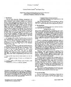
Metadata-to-Data

We use the simple mapping in Figure 2 to test the performance of the generated instance queries. This simple mapping, with one placeholder, allows to clearly study the effect of varying the number of labels assigned to the placeholder. We compare the performance of three XQuery scripts. The first one was generated using a traditional schema mappings and the query generation algorithm in [18]. For each label value in the source, a separate query over the source data is generated by [18] and the resulting target instance is the union of the result of all those queries. The second query script is our two-phase instance query. The third query script is an optimized version of our instance query. If we only use source placeholders, we know at compile-time the values of the source labels that will appear as data in the target. When this happens, we can remove the iteration over the labels in the source and directly write as many return clauses as needed to handle each value. We ran the queries and increased the input file sizes, from 69 KB to 110 MB, and a number of distinct labels from 3 to 600. The generated Input data varied from 600 to 10,000 distinct tuples. Figure 8 shows the query execution time for the three queries when the input had 10,000 tuples (the results using smaller input sized showed the same behavior). The chart shows that classical mapping queries are outperformed by MAD mapping queries by an order of magnitude, while the optimized queries are faster by two orders of magnitude. Again, the example in Figure 2 presents minimal manipulation of data, but effectively shows that one dynamic element in the mapping is enough to generate better queries than existing solutions for mapping and query generation. The graph also shows the effect of increasing the number of distinct labels encoded in the placeholder. Even with only 3 distinct labels in the placeholder, the optimized query is faster than the union of traditional mapping queries: translating 10,000 tuples it took 1 second vs 2.5 seconds. Notice that when the number of distinct labels mapped from the source are more than a dozen, a scenario not unusual when using data exported from spreadsheets, the traditional mapping queries take minutes to hours to complete. Our optimized queries can take less than two minutes to complete the same task.

Implementation Remarks

In our current prototype implementation, we produce instance and schema queries in XQuery. It is worth pointing out that XQuery, as well as other XML query languages such as XSLT, support querying of XML data and metadata, and the construction of XML data and metadata. In contrast, relational query languages such as SQL do not allow us to uniformly query data and metadata. Even though many RDBMS store catalog information as relations and allow users to access it using SQL, the catalog schema varies from vendor-tovendor. Furthermore, to update or create catalog information, we would need to use DDL scripts (not SQL). Languages that allow one to uniformly manipulate relational data-metadata do exists (e.g., SchemaSQL [11] and FISQL [25]). It is possible, for e.g., to implement our relational data-metadata translations as FISQL queries.

EXPERIMENTS

We conducted a number of experiments to understand the performance of the queries generated from MAD mappings and compared them with those produced by existing schema mappings tools. Our prototype is implemented entirely in Java and all the experiments were performed on a PC-compatible machine, with a single 1.4GHz P4 CPU and 760MB RAM, running Windows XP (SP2) and JRE 1.5.0. The prototype generates XQuery scripts from the mappings and we used the Saxon-B 9.05 engine to run them. Each experiment was repeated three times, and the average of the three 5

100

Number of distinct labels

The query above first defines two sets. The first set times is the set of all values under the key attribute time. The second set attributes is the set of all the attributes names in the target instance Stockquotes. For each key value in times, all tuples in the target instance with this key value are collected under a third set called elements. At this point, the query iterates over all attribute names in attributes. For each attribute a in attributes, it checks whether there is a tuple t in elements with attribute a. If yes, the output tuple will contain attribute a with value as determined by t.a. Otherwise, the value is null. It is possible that there is more than one tuple in elements with different a values. In this case, a conflict occurs and no target instance can be constructed.

6.

100

10

Target’ = let times := Target.Stockquotes.time, attributes := dom (Target.Stockquotes) for t in times return [ Stockquotes= let elements := Target.Stockquotes[time=t] for a in attributes return [ if is-not-in (a, elements) then a = null else a = elements.a ] ]

5.4

1000

6.2

Data-to-Metadata

To understand the performance of instance queries for data-to6

http://saxon.sourceforge.net/

269

http://www.cs.toronto.edu/tox/toxgene

100000

10000

1000

Query Execution Time [s]

Query execution time [s]

100000

Data exchange (1) Make hom. (1) Make hom.+merge (1) Data exchange w/Merge (2) Make Hom (2)

100

10000

1000

100

Data exchange + merge + hom. (1) Data exchange w/merge + hom. (2)

10

1 10

0

20000

40000

60000

80000

100000

120000

Number of tuples 1 1000

3000

6000

12000

24000

44000

60000

120000

Figure 10: Performance of MAD mappings for Data-toMetadata exchange.

Number of tuples

Figure 9: Data exchange and post processing performance. Figure 10 compares the total execution times of sets (1) and (2). The time includes the query to generate the target instance and the needed time to make the record homogeneous and merge the result. The results show that optimized queries are faster than default queries by an order of magnitude. Notice that queries in set (1) took more than two minutes to process 12,000 tuples, while the optimized queries in set (2) needed less than 25 seconds.

metadata mappings, we used the simple StockTicker - Stockquotes example from Section 2.3. In this example, the target schema used a single ndos construct. To compare our instance queries with those produced by a data-data mapping tools, we manually constructed a concrete version of the target schema (with increasing numbers of distinct symbol labels). Given n such labels, we created n simple mappings, one per target label, and produced n data-to-data mappings. The result is the union of the result of these queries. The manually created data-to-data mappings performed as well as our data-to-metadata instance query. Notice, however, that using MAD we were able to express the same result with only three value correspondences. We now discuss the performance of the queries we use to do post-processing into homogeneous records and merging data using special Skolem values. In this set of experiments, we used source instances with increasing number of StockTicker elements (from 720 to 120,000 tuples), and a domain of 12 distinct values for the symbol attribute. We generated from 60 to 10,000 different time values, and each time value is repeated in the source in combination with each possible symbol. We left a fraction (10%) of time values with less than 12 tuples to test the performance of the postprocessing queries that make the records homogeneous. The generated input files range in sizes from 58 KB to 100 MB. Figures 9 and 10 show the results for two sets of queries, identified as (1) and (2). The set (1) includes the instance queries (Q1 and Q2 in Figure 5 and labeled “Data exchange” in Figure 9), and two post-processing queries (Q4 ): one that makes the target record homogeneous (labeled “Make hom”), and another that merges the homogeneous tuples when they share the same key value (labeled “Make hom.+merge”). Set (2) contains the same set of queries as (1) except that the instance queries use a user-defined Skolem function that groups the dynamic content by the value of time. The instance queries in (1) use a default Skolem function that depends on the values of time and symbol. Figure 9 shows the execution time of the queries in the two test sets as the number of input tuples increase. We first note that the instance query using the default Skolem function (“Data exchange”) takes more time to complete than the instance query that uses the more refined, user entered, Skolem function (“Data exchange w/Merge”). This is expected, since, in the second phase, the data exchange with merge compute only 1 join for each key value, while the simple data exchange computes a join for each pair of (time, symbol) values. It is also interesting to point out that the scripts to make the record homogeneous are extremely fast for both sets, while the merging of the tuple produced by the data exchange is expensive since a self join over the output data is required.

7.

RELATED WORK

To the best of our knowledge, there are no mapping or exchange systems that support data-metadata translations between hierarchical schemas, except for HePToX [3]. Research prototypes, such as [9, 14], and commercial mapping systems, such as [5, 13, 21, 22], fully support only data-to-data translations. Some tools [13, 21] do have partial support for metadata-to-data transformations, exposing XQuery or XSLT functions to query node names. However, these tools do not offer constructs equivalent to our placeholder and users need to create a separate mapping for each metadata value that is transformed into data (as illustrated in Section 2.2). In contrast to the XML setting, data exchange between relational schemas that also support data-metadata translations have been studied extensively. (See [24] for a comprehensive overview of related work.) Perhaps the most notable work on data-metadata translations in the relational setting are SchemaSQL [11] and, more recently, FIRA / FISQL [24, 25]. [15] demonstrated the practical importance of extending traditional query languages with datametadata by illustrating some real data integration scenarios involving legacy systems and publishing. Our MAD mapping language is similar to SchemaSQL. SchemaSQL allows terms of the form “relation → x” in the FROM clause of an SQL query. This means x ranges over the attributes of relation. This is similar to our concept of placeholders, where one can group all attributes of relation under a placeholder, say hhallAttrsii, and range a variable $x over elements in hhallAttrsii by stating “$x in hhallAttrsii” in the for clause of a MAD mapping. Alternatively, one can also write “$x in dom(relation)” to range $x over all attributes of relation or, write “$x in {A1 , ..., An }”, where the attributes A1 , ..., An of relation are stated explicitly. One can also define dynamic output schemas through a view definition in SchemaSQL. For example, the following SchemaSQL view definition translates StockTicker to Stockquotes (as described in Section 1). The variable D is essentially a dynamic element that binds to the value symbol in tuple s and this value is “lifted” to become an attribute of the output schema. create view DB::Stockquotes(time, D) as select s.time, s.price from Source::StockTicker s, s.symbol D

270

This view definition is similar to the MAD mappings m and c that was described in Section 2.3. (Recall that the mapping m describes the data-to-metadata translation and c is used to enforce the homogeneity/relational model.) A major difference, however, is that the SchemaSQL query above produces only two tuples in the output where tuples are merged based on time. On the other hand, mappings m and c will generate queries that produce three tuples as shown in Section 1. It is only in the presence of an additional key constraint on time that two tuples will be produced. FISQL is a successor of SchemaSQL that allows more general relational data-metadata translations. In particular, while SchemaSQL allows only one column of data to be translated into metadata in one query, FISQL has no such restriction. In contrast to SchemaSQL which is may be non-deterministic in the set of output tuples it produces due to the implicit merge semantics, FISQL does not merge output tuples implicitly. MAD mappings are similar to FISQL in this aspect. However, unlike FISQL which has an equivalent algebra called FIRA, we do not have an equivalent algebra for MAD mappings. Recall, however, that the purpose of MAD is to automatically generate mapping expressions that encode these data-metadata transformation starting from simple lines. In Sections 5 we described how the generated mappings are translated into a query. If our source and target schemas are relational, we could translate those queries into SchemaSQL or FISQL. HePToX [3, 4] is a P2P XML database system that uses a framework that has components that are similar to the first two components of data exchange, as described in Section 1. A peer joins a network by drawing lines between the peer Document Type Descriptor (DTD) and some existing DTDs in the network. The visual specification is then compiled into mappings that are expressed as Datalog-like rules. Hence, these two components of HePToX are similar to the visual interface and, respectively, mapping generation components of the data exchange framework. Although HePToX’s Datalog-like language, TreeLog, can describe data-to-metadata and metadata-to-data translations, HePToX does not allow target dynamic elements. I.e., neither HePToX’s GUI nor its mapping generation algorithm support nested dynamic output schemas. Lastly, the problem of generating a target schema using mappings from a source schema (i.e., metadata-to-metadata translations) is also known as schema translation [17]. The ModelGen operator of Model Management [2] (see Section 3.2 of [1] for a survey of ModelGen work) relies on a library of pre-defined transformations (or rules) that convert the source schema into a target schema. Alternatively, [17] uses mappings between meta-metamodels to transform metadata. None of these approaches, however, allow for data-to-metadata transformations.

8.

erate the mappings and the corresponding queries that perform the exchange. Acknowledgments We thank Lucian Popa and Cathy M. Wyss for insightful comments on the subject of the paper.

9.

CONCLUSION

We have presented the problem of data exchange with data-metadata translation capabilities and presented our solution, implementation and experiments. We have also introduced the novel concept of nested dynamic output schemas, which are nested schemas that may only be partially defined at compile time. Data exchange with nested dynamic output schemas involves the materialization of a target instance and additionally, the materialization of a target schema that conforms to the structure dictated by the nested dynamic output schema. Our general framework captures relational data-metadata translations and data-to-data exchange as special cases. Our solution is a complete package that covers the entire mapping design process: we introduce the new (minimal) graphical constructs to the visual interface for specifying data-metadata translations, extend the existing schema mapping language to handle data-metadata specifications, and extend the algorithms to gen-

271

REFERENCES

[1] P. Bernstein and S. Melnik. Model Management 2.0: Manipulating Richer Mappings. In SIGMOD, pages 1–12, 2007. [2] P. A. Bernstein. Applying Model Management to Classical Meta Data Problems. In CIDR, pages 209–220, 2003. [3] A. Bonifati, E. Q. Chang, T. Ho, and L. V. S. Lakshmanan. HepToX: Heterogeneous Peer to Peer XML Databases. Technical Report CoRR cs.DB/0506002, arXiv.org, 2005. [4] A. Bonifati, E. Q. Chang, T. Ho, L. V. S. Lakshmanan, and R. Pottinger. HePToX: Marrying XML and Heterogeneity in Your P2P Databases. In VLDB(demo), pages 1267–1270, 2005. [5] M. J. Carey. Data delivery in a service-oriented world: the BEA aquaLogic data services platform. In SIGMOD, pages 695–705, 2006. [6] R. Fagin, P. G. Kolaitis, R. J. Miller, and L. Popa. Data Exchange: Semantics and Query Answering. TCS, 336(1):89–124, 2005. [7] M. Friedman, A. Y. Levy, and T. D. Millstein. Navigational Plans For Data Integration. In AAAI/IAAI, pages 67–73, 1999. [8] A. Fuxman, M. A. Hern´andez, H. Ho, R. J. Miller, P. Papotti, and L. Popa. Nested Mappings: Schema Mapping Reloaded. In VLDB, pages 67–78, 2006. [9] L. M. Haas, M. A. Hern´andez, H. Ho, L. Popa, and M. Roth. Clio Grows Up: From Research Prototype to Industrial Tool. In SIGMOD, pages 805–810, 2005. [10] P. G. Kolaitis. Schema mappings, data exchange, and metadata management. In PODS, pages 61–75, 2005. [11] L. V. S. Lakshmanan, F. Sadri, and I. N. Subramanian. SchemaSQL A Language for Interoperability in Relational Multi-Database Systems. In VLDB, pages 239–250, 1996. [12] M. Lenzerini. Data Integration: A Theoretical Perspective. In PODS, pages 233–246, 2002. [13] Altova MapForce Professional Edition, Version 2008. http://www.altova.com. [14] S. Melnik, P. A. Bernstein, A. Halevy, and E. Rahm. Supporting Executable Mappings in Model Management. In SIGMOD, pages 167–178, 2005. [15] R. J. Miller. Using Schematically Heterogeneous Structures. In SIGMOD, pages 189–200, 1998. [16] R. J. Miller, L. M. Haas, and M. A. Hern´andez. Schema Mapping as Query Discovery. In VLDB, pages 77–88, 2000. [17] P. Papotti and R. Torlone. Schema exchange: A template-based approach to data and metadata translation. In ER, pages 323–337, 2007. [18] L. Popa, Y. Velegrakis, R. J. Miller, M. A. Hern´andez, and R. Fagin. Translating Web Data. In VLDB, pages 598–609, 2002. [19] E. Rahm and P. A. Bernstein. A survey of approaches to automatic schema matching. VLDB J., 10(4):334–350, 2001. [20] M. Roth, M. A. Hern´andez, P. Coulthard, L. Yan, L. Popa, H. C.-T. Ho, and C. C. Salter. XML mapping technology:Making connections in an XML-centric world. IBM Sys. Journal, 45(2):389–410, 2006. [21] Stylus Studio 2008, XML Enterprise Suite, Release 2. http://www.stylusstudio.com. [22] Microsoft BizTalk Server 2006 R2. http://www.microsoft.com/biztalk/. [23] C. M. Wyss and E. L. Robertson. A Formal Characterization of PIVOT/UNPIVOT. In CIKM, pages 602–608, 2005. [24] C. M. Wyss and E. L. Robertson. Relational Languages for Metadata Integration. ACM TODS, 30(2):624–660, 2005. [25] C. M. Wyss and F. I. Wyss. Extending Relational Query Optimization to Dynamic Schemas for Information Integration in Multidatabases. In SIGMOD, pages 473–484, 2007. [26] C. Yu and L. Popa. Semantic adaptation of schema mappings when schemas evolve. In VLDB, pages 1006–1017, 2005.

APPENDIX

role is to copy the attributes as elements on the target. MAD produces the following mapping for this specification:

A. DEFINITION OF “CONFORMS TO”

for $x1 in Source.properties, $x2 in hhattrsii let $x3 := $x1 .property.($x2 ) exists $y1 in Target.properties, $y2 in hhnamesii, $y3 in hhelemsii $y4 := $y1 .($y2 ), $y5 := $y1 .($y3 ) let where $y2 = $x1 .property.@name and $y4 .@amount = $x1 .property.pval and $y3 = $x2 and $y5 = $x3

A NR schema T with roots T10 , ..., Tk0 conforms to a ndos schema Γ with roots R1 , ..., Rk if there is a permutation of T10 , ..., Tk0 into T1 , ..., Tk such that Ti conforms to Ri , 1 ≤ i ≤ k. 1. If R is of String type, then T conforms to R if T is of type String. 2. If R is of Int type, then T conforms to R if T is of type Int. 3. If R is of Rcd[l1 : τ1 , ..., lm : τm , $d : τ ] type, then T 0 conforms to R if T is of type Rcd[l1 : τ10 , ..., lm : τm , lm+1 : 0 0 0 τm+1 , ..., ln : τn ] and τi conforms to τi , 1 ≤ i ≤ m, and 0 τm+j conforms to τ , 1 ≤ j ≤ n.

Replacing x2 with a set of literal values, and rewriting to remove $x3 , and $y2 , . . . , $y5 , we obtain a simplified mapping expression: for $x1 in Source.properties, $x2 in {‘@lang’,‘@data’,...,‘@format’} exists $y1 in Target.properties where $y1 .($x1 .property.@name).@amount = $x1 .property.pval and $y1 .($x1 .property.@name).($x2 ) = $x1 .property.($x2 )

4. If R is of Choice[l1 : τ1 , ..., lm : τm , $d : τ ] type, then T conforms to R if T is of type Choice[l1 : τ10 , ..., lm : 0 0 , ..., ln : τn0 ] and τi0 conforms to τi , 1 ≤ i ≤ τm , lm+1 : τm+1 0 m, and τm+j conforms to τ , 1 ≤ j ≤ n.

B.

C.

METADATA-TO-METADATA TRANSLATION EXAMPLE

Unlike data-to-data, metadata-to-data, or data-to-metadata translations, metadata-to-metadata translations are not as interesting as they can always be implemented with the traditional data-to-data translation framework. To see this, consider the example shown below on the left which, essentially, generates a copy of the source schema and instance. This is no different from specifying the exchange as shown on the bottom right. Source: Rcd Target: Rcd Sales: SetOf Rcd Sales: SetOf Rcd month month label USA value UK label Italy

value

Source: Rcd Sales: SetOf Rcd month USA UK Italy

Target: Rcd Sales: SetOf Rcd month USA UK Italy

However, when combined with other data-metadata constructs, we can accomplish complicated mappings with just a few lines. Consider the example in Figure 11. This kind of transformations are not uncommon in many data exchange situations. Source: Rcd properties: SetOf Rcd Target: Rcd properties: SetOf Rcd property: Rcd label1 @name value1: Rcd @lang label @amount @date value label2 … value2 @format pval ...

Figure 11: A more complex example This mapping is expressed with a data-to-meta data combined with a metadata-to-metadata mapping, whose only (but crucial)

272

Algorithm 2 MAD mapping generation Require: a set of skeletons K and a set of correspondences V Ensure: a set of MAD mappings M 1: M = ∅; {For each value correspondence in V } 2: for v ∈ V do 3: {Find all matching skeletons.} 4: for k = (ti , tj ) ∈ K do 5: if source(v) matches ti and target(v) matches tj then 6: Add v to the set of correspondences matched to k. 7: Mark k as “active”. 8: end if 9: end for 10: end for {Remove implied and subsumed mappings} 11: for k = (ti , tj ) ∈ K do 12: {The definition of “subsumed” and “implied” is in [8].} 13: if k is “active” and is subsumed or implied by another active skeleton then 14: Mark k as “inactive”. 15: end if 16: end for {Emit the mappings} 17: for k = (ti , tj ) ∈ K do 18: if k is “active” then 19: m ← a new mapping for skeleton (ti , tj ). 20: Add the expressions in ti to the for, let, and where clauses of m. 21: Add the expressions in tj to the exists, let, and where clauses of m. 22: Use the value correspondences matched to k to create the s-t conditions in the last where clause of m. {An optional simplification of the mappings} 23: m ← rewrite(m) 24: M ←M ∪m 25: end if 26: end for

Algorithm 1 Prepare Mapping Skeletons Require: a source schema S and a target ndos T . Ensure: a set of mapping skeletons. {Compute a set of source tableaux τS .} 1: Visit the schema tree S starting from the root 2: for each set type, choice type, or dynamic placeholder do 3: if visiting a dynamic placeholder hhDii then 4: Let xi−1 be the variable used in the context tableau expression. 5: Create a {xi ∈ hhDii} tableau expression. 6: Add xi+1 := xi−1 .(xi ) to the let clause of the tableau. 7: else 8: if visiting a set or choice type expression gi then 9: Create a {xi ∈ gi } or a {xi ∈ choice gi of L} tableau expression as in Clio [18]. 10: end if 11: end if 12: end for {Compute a set of target tableaux τT .} 13: Visit the schema tree T starting from the root 14: for each set type, choice type, or dynamic placeholder do 15: if visiting a dynamic placeholder hhDii then 16: Let yi−1 be the variable used in the context tableau expression. 17: Create a {yi ∈ hhDii} tableau expression. 18: if the type of hhDii.value is a set type then 19: Add xi+1 ∈ xi−1 .(xi ) to the tableau expression. 20: else 21: Add xi+1 := xi−1 .(xi ) to the let clause of the tableau. 22: end if 23: else 24: if visiting a set or choice type expression gi then 25: Create a {xi ∈ gi } or a {xi ∈ choice gi of L} tableau expression as in Clio [18]. 26: end if 27: end if 28: end for 29: Enhance the source and target tableau by chasing over the parent-child relationships and foreign key constraints (details of this step are in [18]). {Prepare the skeletons.} 30: Create a set of skeletons K = {(ti , tj ) | ti ∈ τS , tj ∈ τT }. 31: return τS , τT , K

Algorithm 3 rewrite Require: a mapping m. Ensure: a simplified version of m. 1: {Remove the let clauses.} 2: for each let clause of the form x := E in m do 3: Replace occurrences of x with E in the where clause. 4: Remove x := E from the let clause. 5: end for {Replace the target-side dynamic placeholders.} 6: for each “x in hhDii” in the exists clause of m do 7: Find an expression x = E in the where clause. 8: Remove that expression from the where clause. 9: Remove “x in hhDii” from the exists clause. 10: Replace x with E in the where clause. 11: end for {Replace the source-side placeholders.} 12: for each “x in hhDii” in the for clause of m do 13: Replace hhDii with a set of literal values {d1 , . . . , dm }. 14: end for 15: return m.

273