Data Driven Refinement of Active Shape Model Search ... - CiteSeerX
Recommend Documents
Active shape model (ASM) statistically represents a shape by a set of well-defined landmark points and models object variations using principal component ...
A.A. Eicherâ, P. Maraisâ, C. Wartonâ , S.W. Jacobson§â â¡, J.L. Jacobson§â â¡, C.D. Molteno§, E.M.. Meintjesâ ¶. âDepartment of Computer Science, University of ...
the point distribution model was first used to learn shape priors of prostate from .... 2D TRUS images by using a novel partial active shape model (PASM) to ...
Based on these security controls security patterns have to be selected. ... Current SOA and cloud services are scattered across multiple heterogeneous security ...
Early evidence that vision can help speech recognition by computer was pre- ... recognition systems, the key lies in a good choice of feature space in which .... tie-clip microphone was adjusted for each talker through a mixing desk and fed.
the resulting model best matches the given silhouette. .... In recent years Seo and Magnenat-Thalmann ..... Measure Technologies for Online Clothing Store", pp.
obtained by using a discrete deformable model with optimal search, which is ... [email protected], 914-945-6138 (phone), 914-945-6330 (fax) .... in order to deal with the shadow artifacts, only the partial salient contour will be .... the exper
ment of Radiology, Leiden University Medical Center, 2300 RC Leiden, The. Netherlands. He is now with ... Color versions of one or more of the figures in this paper are available online ... Region- and edge-based low-level image processing tech- niqu
Keywords: Active Shape Model, segmentation, shape constraints, statistical shape ... Our shape energy term does not require additional parameters, whereas ...
We propose a new deformable shape model Active Shape Structural ... by Mitchell et. al [2] extends the active appearance model to fit a time varying shape.
A Multi-View Nonlinear Active Shape Model. Using Kernel PCA. Sami Romdhanif , Shaogang Gong% and Alexandra Psarrouf f Harrow School of Computer ...
Active Shape Model is an efficient way for localizing ob- jects with variable shapes. When ASM is extended to multi- view cases, the parameter estimation ...
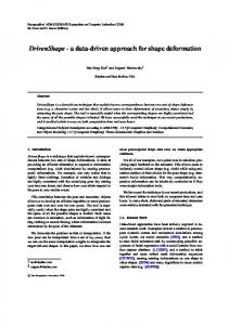
DrivenShape - a data-driven approach for shape deformation. Tae-Yong Kimâ ... used to reconstruct final position df in
Meinzer observe in their recent review [5] that nonlinear, landmark-based ... squares projection in Eq. 1, this approach does not guarantee a result which is.
Detecting Facial Features Using Active Shape Model. Abdulganiyu Abdu Yusuf 1*, Zahraddeen Sufyanu2. 1,2Faculty of Informatics and Computing, 21300 Gong ...
CURTIS C., MAIGRET E., PRASSO L., FARSON P.: An art-directed wrinkle system for cg character clothing and skin. Graphical Models 69, 5-6 (2007), 219â230.
PCA is still unsmooth when the shape has a large variation compared with the mean ...... Sparse Data. 3D. Data Processin
locating a landmark. ai equals to 0 implies that classifier can perfectly predict shape's boundary; while ai equals to 1
Penn 87, Smit 87], since they provide more powerful constructs for structural and behavioral ..... If no teller is free, customers line up in a common queue.
After the executable file .... [Penn 87] D. Penney and J. Stein, Class Modification in the GemStone Object-Oriented Database System, OOPSLA '87 Conference ...
cheap flights? 2. OVERALL ARCHITECTURE AND. EXECUTION FLOWS. Within the multi-domain query answering problem we identify two main activity flows: ...
In McCracken et al (2001) the authors found âshockingly low performance on ... encompass gender (Sanders 1998), the educational level of parents (Ting & Robinson. 1998) ACT/SAT ... Horstmann, C.S., Big Java, John Wiley & Sons, 2001.
Instructing the computer: The programming language is viewed as a high-level ... When designing a programming course one decides how much time, effort and focus ..... programs with a good structure, low coupling and high cohesion.
Data Driven Refinement of Active Shape Model Search ... - CiteSeerX
Active Shape Models (ASMs) [1,2] provide a useful means for locating ... To search for an object using an Active Shape Model an initial estimate of the sol.
Data Driven Refinement of Active Shape Model Search T.F.Cootes and C.J.Taylor Department of Medical Biophysics, University of Manchester Manchester M13 9PT
Abstract Active Shape Models (ASMs) provide an efficient means of locating ob jects in images. By statistically modelling the shape variations in a class of objects they can rapidly and robustly fit to new examples. However, if an ASM does not represent all the shape variation exhibited by the object, the model may not be able to locate new examples accurately. This paper describes two complementary approaches to allowing additional freedom to the points which compromise the model, enabling them to fit to the image data more accurately. We present results for synthetic and real images and discuss how the methods can be used in an interactive ‘boot strap’ training scheme where problems with over-constrained models are particularly important.
ÁÂÄÀÅÃÇÉÊËÅÈÇÀ
Active Shape Models (ASMs) [1,2] provide a useful means for locating objects in images. An ASM relies on having statistical models of the expected shape and greyÁlevel appearance of the object of interest, generated from training images. It represents an object as a set of model points, typically located on the object bound aries, each with an associated greyÁlevel model of the surrounding region. To search for an object using an Active Shape Model an initial estimate of the sol ution is iteratively refined. At each step the greyÁlevel models associated with each point are run along normals through current positions, and the best match found. The model parameters are then updated to move the model points toward these suggested positions. Because the model points can not move independently, only in ways determined by the shape model, they do not necessarily end up exactly at the point which best fit the greyÁlevel model. This constraint is important during the search, where it helps gives rapid and robust convergence, but sometimes leads to unsatisfactory results. There are two reasons for the model points not fitting the data exactly when the search has converged correctly. One is that the shape model does not contain enough variability to express the full range of deformations the target can exhibit (Figure 1). This is commonly the case when a model has been built from a small number of training examples. Secondly errors can be caused by noise and clutter which give false responses from the greyÁlevel models, distracting the shape model from the correct solution (Figure 2). The latter example shows
that simply moving to the best candidate point is unlikely to work except in noise and clutter free images. Model Point Best Found Point
Model Point Best Found Point Other Found Points
Figure 1 : Because the shape model does Figure 2 : A strong noise edge can attract not include a ‘bending’ mode of vari one point, leading to a compromise sol ation, a leastÁsquares compromise posi ution for all the points. tion is found.
A multiÁresolution search technique [2] can reduce the effects of spurious feature responses (by gradually reducing the length of the search profile) but does not help with an overconstrained shape model. In this paper we describe two complementary methods which allow the model points freedom to move away from their current model constraints to fit the image data more accurately. One is to artificially add extra variation to the model in a way which encourages smooth deformations away from the original model. The second is to allow the model points to move directly to the set of candidate positions which is most consistent with the current shape model. We determine this set by a depthfirst tree search of all the possible sets. This combinatorial approach is necessary to overcome problems with false responses from the feature detectors. Problems of inaccuracy are particularly prominent when we are labelling images to train a model. To mark points manually is time consuming and tedious. An appeal ing approach is ‘bootstrap’ the model, using a model trained on the first few example images to help locate the points in the subsequent images. However, though this can speed up the annotation considerably, it still requires a great deal of user interaction to adjust points which are not fitted well (which in the early stages of training can be almost all of them). A more data driven approach to adjust ing the points to better fit the images could help the user considerably and signifi cantly reduce the time required to mark up a training set. 2 Related Work
Locating rigid objects by finding plausible sets of features has been explored by many authors, including Grimson [3], who gives a comprehensive literature survey. Locating approximate positions for flexible objects by finding sets of distinctive fea tures is discussed by Cootes and Taylor [4]. Feature detectors are run over the whole image and shape models are used to find plausible combinations of features to initialise Active Shape Models. The current work uses a similar methodology,
but concentrates on locating model points accurately, given an initial approximation obtained by ASM search. Isard and Blake [5] overcome the problem of clutter in a tracking problem by track ing a set of possible solutions, each of which is tested against the image and assigned a probability depending on the quality of fit. At each iteration of a tracking algo rithm a new set of solutions is generated by sampling from the old set and deforming each sample by perturbing a random amount drawn from a known distribution. This favours solutions with good image evidence and biases against those which have just latched on to some clutter. The approach appears to give good robust approximate solutions, but since it simply detects the nearest edges may not be appropriate for interpreting static images where accuracy is important. Cootes and Taylor [7] addressed the problem of adding extra variation in the form of the modes of vibration of a finite element model based on the training shapes. The approach we take here is simpler and allows a more intuitive choice of the amount of extra variation to allow. One approach to refining the fit of a boundary model to image data is to use an Ac tive Contour (or ‘snake’) [8]. However, snakes impose arbitrary constraints on boundary smoothness (so may still be prone to clutter biasing their position) and do not easily allow general shape constraints to be imposed. The behaviour of Ac tive Shape Models is similar to that of snakes, but allows explicit constraints based on statistical shape models to be applied. 3 Statistical Shape Models
Given a training set of shapes, each represented by n labelled points, we can find the mean configuration (shape) and the way the points tend to vary from the mean [1]. The approach is to align each example set into a common reference frame, represent the points as a vector of ordinates in this frame and apply a principle com ponent analysis (PCA) to the data. By using a subset of the eigenvectors of the cova riance matrix we obtain a shape model x, (1) x = x + Pb + r where  Á ÂÄÀÅ ÃÇÃÇÃÇÃÅ ÄÉÅ ÊÀÅ ÃÇÃÇÃÇÃÅ ÊÉËÈ , P is a 2n x t matrix of eigenvectors of the covariance matrix, S, of a training set, and r is a set of residuals whose variances, ÍÎ , are deter mined by cross-validation. b is a vector of t shape parameters, where t is chosen so that the model can approximate the original training set to a desired level of accu racy. Each shape parameter ÏÌ has a variance (about zero) of ÑÌ , the ith eigenvalue of the covariance matrix. The quality of fit of a new shape, x, to the model is given by Ú b Ü ÎÛÜÉ rÜ Ì +Š Î È fÓÔÖÒÕ = Š (2) r = x - (x + Pb) b = P (x - x) Ù ÌÛÀ Ì ÎÛÀ vÎ In the case of missing points, we can reformulate this test using weights (1.0 for point present, 0.0 for point missing);
fshape
=
Á t
i=Ä
biÀ Ái
+
Á
j=Àn j=Ä
wi
rÀj vj
where in this case  is obtained as the solution to the linear equation (ÄTÀ)(Å - Å) = (ÄTÀÄ) (À is a diagonal weight matrix).
The points, Å, of an Active Shape Model are controlled by the shape parameters, using (5) Å = Å + ÄÂ This allows only patterns of variation seen in the training set. If the training set is not representative of the variation exhibited by the class of objects, or if the trun cation of the number of modes used (t) is too severe, the model will not necessarily fit exactly to a new example. The columns of the matrix Ä, which represent the modes of variation in the shape model, are the eigenvectors of the covariance matrix of the (aligned) training examples. Cootes and Taylor [7] suggest adding extra variation by adding to ma trices, , determined from the modes of vibration of finite element models based on the training examples. New modes are then generated as the eigenvectors of this augmented covariance matrix. The calculation of the matrices is relatively complex and the proportion that should be added to is not well defined. A simpler approach, which achieves the same aim of allowing smooth deformations, is to in troduce additional variance and covariance directly to . If points i and j are neigh bours along a boundary, we expect them to be coupled and thus their ordinates to have a positive covariance. By adding some value c to the appropriate elements of we can allow the points more freedom to vary, but ensure that neighbouring points tend to vary together. The magnitude of c is the additional variation we wish to allow each point. For example, consider a shape model trained on the three 40 point rectangles shown in Figure 3. These have unit height and varying widths. The model would have a single mode which varied the aspect ratio of the shapes. If we add 0.1 to the diagonal (variance) and off diagonal (covariance) elements representing neighbouring points in the covariance matrix, the modes of variation of the model allow a wider range of shape deformations, favouring smooth deformations (Figure 4). If we performed ASM search with such an augmented model, we would expect to get a better fit to the data. However, the less constrained model would be less likely to converge to the correct solution from a poor starting position, since it would be more likely to latch on to the wrong structures in the image. In practice, the original model should be used to obtain an initial estimate, then the augmented model run from this position to refine the fit. The number of modes used by the augmented model should be at least t (the original number of modes) but not so many as to allow Â,
Figure 3 : Training set of rectangles Mode 1
Mode 5
Mode 4
Mode 7 Figure 4 : Some modes of shape variation of rectangle model with augmented covariance matrix
very distorted shapes. The best choice for this number is currently the subject of investigation. 5 Dealing With Clutter
When we truncate the shape model it will still not fit exactly to all examples we en counter. Also it will still be prone to noise and clutter pulling it away from the opti mal point positions (Figure 2). If we assumed that the grey-level models were able to locate the best point positions along the normals we could simply move each model point to the best matching position. This would tend to give a satisfactory solution given a good enough initial match, except in regions of high boundary cur vature, where the true image points might not lie along the normals. However, in practice there are often spurious responses from the greyÁlevel models (eg caused by strong nearby edges) which would cause such a naive scheme to fail (Figure 2). If we assume that the true position for each model point is one of the points along the normal, but may not be the one with the best response to the grey-level model, we need an alternative way of picking it out. Rather than treat each point individ ually, we will consider them as a set, and pick out the candidate for each model point which belongs to the set of points which is most plausible given the current shape model. 6 Testing Sets of Points
We wish to test plausibility of a set of image points which form a shape, X, as an example of shape model. To do this we calculate the shape parameters b and the pose Q (mapping from model frame to image) which minimise the distance of the transformed model points, X’, to the target points (6) X Á XÂ = Q(x + Pb) ( Q is a 2D Euclidean transformation with four parameters, ÅÄ ÃÇÅÀ ÇÃÇÉ and ÅÃÇ
This is a straightforward minimisation problem [1]. Having solved for Q and b we can project the points into the model frame using QÊË and calculate the residual terms and hence the quality of fit, fÁÂÄÀÅ , using Eq. 3. There are several tests we could apply to determine if the points X were an accept able combination. 1. We could impose a hard limit on fÁÂÄÀÅ (which could be estimated from its prob ability distribution) 2. We could impose limits on the allowable pose parameters in Q. 3. We could impose limits on the shape parameters, b (for instance Ã Ç ËÉÊ ). 4. We could impose limits on the residuals either in the image frame or in the model frame. In the last case we may wish to limit solutions to those whose points vary by no more than a given number pixels from the best fit with the current model (to restrict the extra variation allowed). The residual error is given by (7) R = X - XÈ = X - Q(x + Pb) We can then test the residual error on each point. In practise we have found constraints 3 and 4 (limits on shape parameters and resid uals) to be the most useful. To compare sets of points, apply these tests; of those sets which pass we choose that with the lowest fÁÂÄÀÅ . ÍÎÏÌÑÌÓÔÖÒÕÎÔŠÌÎÚÌÛÔÎÏÌÔÎÜÙΟŽÒ Ö ŽÔÌÎ ÜÖÒÔÛ Suppose we have run an ASM to convergence on an image, then used the grey-level model for each model point to locate a number of new candidate positions along profiles normal to the boundary through the points (Figure 5). These candidates are generated by finding peaks in responses of the grey level models when moved along the normals. In the simplest case they give the positions of nearby edges. Model Points Candidate Points True Target Figure 5 : Having run an ASM to convergence we locate candidates for each model point along their normals. Clutter and noise cause spurious responses.
We wish to find the combination of candidate points which gives the best match to the shape model. For anything more than a very small number of points and candi dates, exhaustive search is prohibitive, requiring ! "Ê tests (if the ith of the n points has mÊ candidates, or more if we consider the case where some true positions are missing. However, the optimum solution can be reached using a pruned depth first tree search. In advance we build statistical shape models for sub sets of the first 2,3,..n points. The candidates for each are sorted by quality of fit and,
if missing features are to be allowed, a wildcard is added. We then recursively con struct sets, starting with a candidate for the first point and adding each candidate for the second in turn. The quality of fit of the pair to the model is tested as de scribed above, and if a pair passes the tests, each candidate for the third point is added and the three points tested. Those sets which pass are extended with candi dates for the fourth and so on. In this manner all possible plausible sets can be gen erated efficiently. (This approach has the advantage that it can be implemented in a recursive algorithm in a small number of lines of code). We record all the com plete sets which have at least three valid points and pass the shape tests. Of these we choose the one with the best quality of fit (ie the smallest shape ). f
8 Example Using Synthetic Data
We have tested the approach using synthetic data. Figure 6 shows the set of points, one chosen from each vertical profile, which best match a straight line model in the presence of many noise responses. This works well, even though the points on the true line are corrupted by significant noise. Figure 7 shows the results of a similar experiment showing a straight line model fitting to curved data (simulating an un dertrained model). In this case the model picks out a number of spurious responses, as they give a more convincing straight line. If we augment the model with extra covariance, allowing it to deform smoothly, we achieve better results (Figure 8). Best set of points Best model fit to points matching shape model
ÈÍÎÏÌÑÓ8Ó:ÓÔÑÖÒÓÖÑÒÓÕŠ ÚÕÍÛÒÖÓÜÙÒŸŽÍÛÎÓÙÓÜÕÌÑ ÌÑ Ù$Ñ Ó ÍÛÑÓÜÕ Ñ
Although this synthetic problem could probably be tackled effectively with dynamic programming, such an approach only takes into account local information, and can not find the set which optimises a global shape-based measure.
9 Examples on Real Images
ÁÂÄÀÅÃÇÉÊÅËÈÊÁÃÍÎÊÂÇÊÀÊÏÀÄÈÊÌÑÀÉÈ Given a shape model of a face, we can use it to locate the facial features in a new image. However, until the shape model is fully trained it will not be able to fit accu rately to new image data. Figure 9 shows the model points representing the lips, after fitting the full face model to an image. The points are approximately correct,
but in some cases are about 5 pixels from the optimal solution. Figure 10 shows profiles constructed through the points on the lower edge of the bottom lip, and indicates the candidate positions for the points. These consist of all peaks in re sponse of the greyÁlevel model at each model point (no threshold is applied). The model points have been moved to the best response in each case. At two of the points this has lead to a poor solution, where the true position has not given the best response. Figure 11 shows the set of points which best match a slightly relaxed version of the shape model for the bottom lip (about 0.1 pixel additional variance has been added). Results for the other lip boundaries could be improved in the same way.
Figure 9 : Initial model points for lips after fitting full model to whole face. Noise and constraints of model prevent points moving to optimal positions
Figure 10 : Candidates for each model point found by searching along normals. The points are moved to the best response, which is not always the desired position.
Figure 11 : Selecting the set of points which are most consistent with the shape model gives a more satisfactory result.
Locating The Thumb in a Hand Image We applied a similar technique to refining the position of the thumb part of a hand model when fit to a hand image (Figures 12-14). The model points for the fingers can be refined in the same way.
Figure 12 : Results of running ASM
Figure 13 : Candidates for each model point found by searching along normals. The points are moved to the best response.
Figure 14 : Selecting the set of points which are most con sistent with the shape model gives a more satisfactory result. 10 Practical Considerations
We are concentrating on developing a semiÁautomatic system for helping the user mark points on a training set. To be useful the methods must achieve their results at least as fast as the user could by manual editing. Calculating the relaxed model requires computing the eigenvectors of the full covariance matrix, which is an %Á&ÂÄ problem and becomes prohibitive for large numbers of points. Calculating the optimal set of points is a combinatorial problem of exponential complexity. However, in practice the user will concentrate on refining one sub-part of the model at a time. We can build models of small sets of points and test combinations of candidate features for these sets sufficiently rapidly to be useful. The current methods do not always produce a satisfactory result and are certainly not robust enough for a fully automatic system. However the results are good enough for an interactive system in which the user can correct poor answers. In practice moving the model points to the best fit along a profile often gives the de sired solution. When it does not the user can invoke to combinatorial search, which
produces a ranked set of possible solutions. The user can rapidly look at each to choose the most suitable, or can edit the points by hand if that is easier. The key parameters of the methods, how much additional variance to add and the acceptable deviation of found points from the best model fit can both be expressed simply in terms of units of distance in the image. This allows the user to make an educated guess at suitable values for a particular problem. 11 Discussion and Conclusions
The combinatorial method relies on the true point position lying along the profile and being successfully located by the grey-level model for that point. Where there is significant noise this may not be the case. To get the best positions we should rely on the averaging effects of the original shape model applied to whole sets of points, and not attempt to adjust the points further. In an interactive system the user can usually decide whether the data is good enough to attempt to improve the model fit. It is not clear whether it will be possible to determine this automatically. Adding extra covariance to to ‘relax’ the shape model and choosing sets of candidate point positions which best match the model are useful techniques for helping a user fit a shape model accurately to an image. This can speed up the generation of train ing sets for more comprehensive statistical models which should be able to fit to the data well with no user interaction. We are investigating ways of achieving robust results when the errors at the convergence of the ASM are small, with a view to producing a fully automated system. References
[1] T.F.Cootes, C.J.Taylor, D.H.Cooper and J.Graham, Active Shape Models Their Training and Application.Computer Vision and Image Understanding Vol. 61, No. 1, 1995. pp.38-59. [2] T.F.Cootes , C.J.Taylor, A.Lanitis, Active Shape Models : Evaluation of a Multi-Resolution Method for Improving Image Search, in Proc. British Machine Vision Conference, (Ed. E.Hancock) BMVA Press 1994, pp.327-338. [3] W.E.L. Grimson. Object Recognition By Computer : The Role of Geometric Constraints. Pub. MIT Press, Cambridge MA, 1990. [4] T.F.Cootes, C.J.Taylor. Locating Objects of Varying Shape Using Statistical Feature Detectors. Lecture Notes in Computer Science: 1065. Computer Vision ECCV’96, (Eds. B.Buxton, R.Cipolla) Springer-Verlag 1996, pp.465-474. [5] M.Isard and A.Blake. Contour Tracking by Stochastic Propagation of Condi tional Density. Lecture Notes in Computer Science: 1065. Computer Vision ECCV’96, (Eds. B.Buxton, R.Cipolla) Springer-Verlag 1996, pp. 343-356. [6] A.Hill, T.F.Cootes, C.J.Taylor. Active Shape Models and the Shape Approxi mation Problem. in Proc. British Machine Vision Conference 1995. Vol.1. (Ed. D.Pycock) BMVA Press. pp. 157-166. [7] T.F.Cootes, C.J.Taylor, Combining point distribution models with shape mo dels based on finite element analysis. Image and Vision Computing Vol. 13, No. 5 June 1995. pp.403-409. [8] M. Kass, A. Witkin and D. Terzopoulos , Snakes: Active Contour Models, in Proc. First International Conference on Computer Vision, pp 259-268 IEEE Comp. Society Press, 1987.