We propose a new deformable shape model Active Shape Structural ... by Mitchell et. al [2] extends the active appearance model to fit a time varying shape.
Generalizing the Active Shape Model by Integrating Structural Knowledge to Recognize Hand Drawn Sketches Stephan Al-Zubi, Klaus Tönnies Otto-von-Guericke University Magdeburg, Department of Simulation and Graphics P.O.Box 4120, D-39106 Magdeburg, Germany {stephan, klaus}@isg.cs.uni-magdeburg.de
Abstract. We propose a new deformable shape model Active Shape Structural Model (ASSM) for recognition and reconstruction. The main features of ASSM are: (1) It describes variations of shape not only statistically as Active shape/Appearance model but also by structural variations. (2) Statistical and structural prior knowledge is integrated resulting in a multi-resolution shape description such that the statistical variation becomes more constrained as structural information is added. Experiments on hand drawn sketches of mechanical systems using electronic ink demonstrate the ability of the deformable model to recognize objects structurally and reconstruct them statistically.
1 Introduction Shape representation, recognition and classification is used for analyzing 2-d and 3-d data as well as to analyze 3-d data from 2-d projections. This work is interested in the former. Various deformable shape models have been developed in recent years and used for segmentation, motion tracking, reconstruction and comparison between shapes. These models can be broadly classified into three paradigms: 1. Statistical models use prior knowledge about shape variation for reconstruction. 2. Dynamic models fit shape data using built-in smoothness constraints. 3. Structural models extract structural features to compare and classify shapes. One of the important statistical models is the Active Shape and Appearance Model developed by Cootes et. al [1] that utilizes principal component analysis in order to describe variations of landmarks and textures. The Active Appearance Motion Model by Mitchell et. al [2] extends the active appearance model to fit a time varying shape like the heart. Another important example is probabilistic registration by Chen [3] that uses the per-voxel gray level and shift vector distributions to guide a better fit between the brain atlas and brain data. The restriction in statistical models is that they describe the statistical variations of a fixed-structure shape and not structural differences between different shapes. An example of dynamic models is the front propagation method by Malladi et. al [4] that simulates an expanding closed curve that eventually fits the shape boundaries. A similar concept is found in dynamic particles by Szeliski et. al [5] that simulate a
system of dynamically oriented particles that expand into the object surface guided by internal forces that maintain an even and smooth distribution between them. Another approach are T-snakes / surfaces by McInerny et. al [6] that use the ACID grid (a decomposition of space) that enable traditional snakes to adapt to complex topologies. The dynamic models are able to segment and sample shapes of complex topology such as blood vessels. Their restriction is that they cannot characterize the shapes they segment either statistically or structurally. A good example of structural models is segmentation of shapes into geons as in Wu et. al [11]. This model uses the finite element method to estimate the charge density of a shape surface. This identifies boundaries of high curvature where the shape is divided into subparts. Seven parametric geons such as cylinder or ellipsoid are fitted to the subparts resulting in a simplified structural description of the shape. A similar concept to geons is shape blending by DeCarlo et. al [8]. It begins by fitting an ellipsoid to the shape. The fitting process tears the surface into two blended surface patches at points where the object has protrusions or holes. The importance of blended surfaces is that we can construct a shape graph of protrusions and holes. Shape structure can also be extracted using the shock grammar by Siddiqi et. al [7]. This model defines four types of shocks, which are evolving medial axes formed from colliding propagating fronts that originate at shape boundaries. The model defines a shock grammar that restricts how the shock types can combine to form a shape. The grammar is used to eliminate invalid shock combinations. Resulting shock graphs facilitate comparison between shapes. The structural models are data driven in that they have no prior knowledge about shape structure. They also can not describe the shapes they fit statistically. The model we propose defines multi-resolution a-priori knowledge about the shape both at the structural and the statistical level. It is called Active Shape Structural Model (ASSM). It extends the ability of statistical models to handle structural variability and structural models to include a-priori shape information.
2 Method Hand drawn sketches were chosen to demonstrate the ASSM because they have the following properties: 1. Sketches are more suitable for shape oriented models as opposed to feature oriented models such as cursive hand writing recognition. 2. Training and testing data are easy to generate and no preprocessing or postprocessing steps are required. 3. If we impose the constraint that no structure is smaller than a stroke, we can easily separate shape sub-structures from each other. 4. Strokes are suitable for statistical analysis because they vary shape in relationship to each other or when drawn by the same user or different users. Sketches are gaining increased importance with the shift to pen based interface used for palm and tablet computers. Currently sketching systems are employed in the field of design such as: Design of user interfaces [13], recognition of mechanical designs [14] and content based image retrieval [12, 15].
7
A3 A1
A4
B1 A2
B2
Fig. 1. Levels of a sketch: (1) Strokes {A1… A4, B1, B2} (2) Objects: Cart, spring (3) Relations: Correlation between the length of the spring and the distance between the cart and the wall.
Fig. 3. Left, middle: the first two variation modes of a rectangle object. Right: The first variation mode of a chair relation between four rectangles. The variation of each rectangle becomes more constrained and correlated to other rectangles.
Fig. 2. The effect of varying the first three shape parameters of a two-stroke shape by ±3 standard deviations.
Fig. 4. A chair modeled as a relation between rectangular single-stroke objects. PCR constructs the expected shape given 1, 2 and three regressor objects from left to right respectively. As we can see regression improves its fit to the original data as more regression objects are used.
Many sketching systems restrict sketch recognition to simple shape primitives such as a square, circle, polygons or other specific shapes [14,16]. We propose a new system that studies sketches statistically allowing a richer, more complex and uniform characterization of shapes. The sketch is represented at three levels: Stroke, object and relation (See Fig. 1). The stroke is the atomic unit of shape. An ordered list of strokes representing a single entity is an object. Groups of objects, that are statistically correlated together, are combined by relations. A relation may also include other relations. The components of a relation are not drawn in any predefined order. The ASSM consists of a training module and a recognition module. The training module provides prior knowledge to the ASSM. The recognition module uses the prior knowledge of the ASSM to recognize and reconstruct structures from sketches. 2.1 The Training Module A shape table is constructed from shape samples in four steps: 1. Strokes and multi-strokes are sampled into statistical vectors. 2. Sampled vectors are aligned for statistical analysis. 3. Principal component analysis is applied on the aligned samples. 4. Shape regression parameters are computed for relations. During sampling, a stroke is defined as a parametric B-spline curve interpolating a sequence of device sampled points: p(t)=(x(t), y(t)) where 0 t tmax is the time in milliseconds. Time is used as the interpolating variable because it samples more of
the curve at points of high curvature and high detail. An n-sampling of the stroke p is a vector xn=(x1, x2 … xn, y1, y2 … yn)T where (xi, yi)=p((i-1)tmax / (n-1)), 1 i n. Objects and relations consist of multiple strokes q=(p1, p2 … pm). q is statistically sampled by concatenating the corresponding sample vectors x=(x1T, x2T … xmT )T. A population of stroke / multiple-stroke samples S={x1, x2 … xp} is then iteratively aligned to an average shape x by finding the transform parameters θi that minimizes the average Euclidian distance between the corresponding n points of xi and x . x is initialized as x1 and recalculated after every realignment of S. The transformation parameters θ are translation and optionally rotation, scale or all three. After aligning S, we apply principal component analysis to yield a matrix of t principal components Φ=[φ φ1, φ2 … φt]. The shape parameters are described by a vector b such that x = x + b . Fig. 2 shows the first three variation modes of a complex two-stroke shape analyzed from 20 samples. The variation of an object becomes more specific as it becomes a part of a relation. Fig. 3 shows how the variation of a rectangle becomes more constrained as it becomes part of a shape group. The significance of this is that a sub-shape changes its variation modes according to its context. Relations can be used to predict new shapes when only some are given using a regression technique. This speeds up searching for relations and also completes missing structures in the image. Principal component regression (PCR) uses the shape parameter space b as regression and observation variables. Shape coordinates x are not used because they have a high linear correlation. Given a relation R = {r1 , r2 ,...rn } between n objects/relations of which A ⊂ R are regression objects and B ⊂ R, B ∩ A = φ are observation objects and given a population of p samples, we compute a regression matrix B as follows: 1. We align the p samples and compute (x, A , B , A , B ) where ( A , A ) are �
�
�
�
the latent vectors and roots of the regressors and similarly ( B , B ) are the latent vectors and roots of the observation objects. 2. For every sample xi, 1 i p compute the shape coordinates of regressors and observation objects b i, A = t (x i, A − x A ), b i, B = t (x i, B − x B ) .
[ b ] and an ] . Then we compute T T p. A
3. We form a regression matrix from shape parameters R = bT1, A
[
observation matrix of shape parameters S = bT1, B
bTp , B
the regression matrix B = (R t R)−1 R t S . Let
= (x,
�
A/ B
the regression parameters of A to B. 4. For a relation R that consists of n objects/relations {r1 regression parameters
�
{r1 , r2
ri −1 } /{ri } ,
i=2
T
�
x,
�
y,
�
x,
�
x , B)
be
rn } we compute the
n.
Fig. 4 shows how PCR is used to predict parts of a chair. We see the match between actual and predicted shapes increases as more shapes are used for regression. The statistical and regression parameters of strokes, objects and relations are then stored in a shape table. For a relation consisting of n objects, regression matrices are stored as {B2 … Bn-1} where Bi means that we use the first 1 ... (i-1) objects as regression shapes and the ith object as the observation object (as depicted in Fig. 4).
2.2 The Recognition Module After constructing the shape table, we can use it to recognize and reconstruct new sketches. The sketch interpretation consists of the following: Sequences of strokes are classified as candidate objects. Then, relations are recognized in the sketch by using the structural prior knowledge to generate new objects given an existing object set. The sketch is then searched for evidence that supports the generated assumption. When there is sufficient data to support the relation then it gets accepted. Finally, conflicting interpretations between candidate objects are resolved using the object’s largest context principle. This means that candidate objects that belong to bigger relations are favored to single objects or objects that belong to smaller relations. Once a candidate object is selected for removal , all the relations it belongs to are removed. The best fitting shape x ′ for a shape class with parameters ( x, , ) and nsampled stroke/object/relation x is computed as follows: 1. Initialize the best fitting model x′ to x . 2. Transform x with rigid body transform into x to minimize x′ − x . �
�
�
�
3. Compute the nearest fitting shape parameters b = (x − x) . 4. Compute the best fitting shape as x′ = x + b . 5. Goto (2) and repeat until x′ converges. The shape similarity measure computed from the best fitting shape x ′ as the weighted sum of the deviation of x ′ from its mean and the maximum distance between the corresponding points of x and x ′ as follows dissimilar ity (x, x, , ) = deformation(x, x, , ) + α ⋅ distance(x, x, , ), (1) T
�
�
�
�
�
�
�
deformation(x, x, , ) = �
�
t
bi
i =1
λi
�
�
�
2
where b =
t �
(x ′ − x) = (b1 , b2 ...bt ) ,
distance(x, x, , ) = max ti =1 x i' − xθ ,i where �
x ′ = ( x1 , x 2
�
x n ), x = ( xθ ,1 , xθ , 2
xθ ,n )
�
Objects and relations are accepted or rejected by applying a threshold τ to eq. 1. Ordered sequences of strokes are classified into candidate objects. Given a sequence of strokes (s 1 , s 2 s k ) we find candidate objects as follows: 1. For every i=1…k, we classify the first {s i , s i + 1
s i + k } strokes for some k using
the shape table ST. We designate C (s j ) as all single stroke classes of which the dissimilarity is below the threshold τ in eq. 1. 2. Every object that starts with a stroke sequence in C (s i ) × C (s i + 1 ) C (s i + k ) is tested by similarity measure in eq. 1 to find the set of acceptable candidate objects CO = {o1 , o2 om }
A relation R = {r1 , r2 rn } with PCR parameters { 1 , 2 n −1 } is recognized by comparing the generated expected object or relation with the actual objects or relations (as depicted in Fig. 4) in the sketch as follows: �
�
�
1. Find all objects of type r1 in the sketch. Set i=2. 2. Generate the expected shape of type ri +1 , call it x′i +1 , using regression parameters 3. Find
�
i and
objects
previously found shapes P = {x1 , x 2 ,
or
relations
of
type
xi } .
ri +1 : S = {x1 , x 2
xk } .
Find
min x j ∈S x j − x′i + 1 4. If x j − x′i + 1