data mining techniques to classify astronomy objects - Researcher

DATA MINING TECHNIQUES TO CLASSIFY ASTRONOMY  OBJECTS Project Report Submitted by

V.SUBHASHINI

Under the guidance of

Dr. Ananthanarayana V. S. Professor and Head Department of Information Technology

DEPARTMENT OF INFORMATION TECHNOLOGY NATIONAL INSTITUTE OF TECHNOLOGY KARNATAKA SURATHKAL – 575 025, INDIA 2008­2009

Acknowledgment

I express my heartfelt gratitude to Dr.Ananthanarayana.V.S, HOD, Department  of Information  Technology,  NITK Surathkal for his invaluable guidance, encouragement and support  throughout this project.  

 

V. SUBHASHINI Student,  B.Tech Dept. of Information Technology NITK, Surathkal

ABSTRACT Astronomical images hold a wealth of knowledge about the universe and its origins; the archives of such  data have been increasing at a tremendous rate with improvements in the technology of the equipments.  Data mining would be an ideal tool to efficiently analyze these enormous datasets, help gather useful  patterns and gain knowledge. Data mining tools for clustering, classification and regression are being  employed by astronomers to gain information from the vast sky survey data. Some classical problems in  this regard are the star­galaxy classification and star­quasar separation that have been worked upon by  astronomers   and   data   miners   alike.   Various   methods   like   artificial   neural   networks,   support   vector  machines,   decision   trees   and   mathematical   morphology   have   been   used   to   characterize   these  astronomical objects.  We first make a study of clustering and classification algorithms like Linear Vector Quantization, Multi­ Layer Perceptrons, kd­trees, Bayesian Belief Networks and others that have been used by astronomers to  classify celestial objects as Stars, Quasars, Galaxies or other astronomical objects. We then experiment  with some of the existing datamining techniques like Support Vector Machines, Decision Trees and  DBSCAN (Density Based Spatial Clustering with Noise) and explore their feasibility in clustering and  classifying astronomy data objects. Our objective is to develop an algorithm to increase the classification  accuracy of stars, galaxies and quasars and reduce computation time. We also compare how the use of  different distance measures and new parameters affect the performance of the algorithm. Thus we also  try to identify the most suitable distance measure and significant parameters that increase the accuracy  of classification of the chosen objects.

3

Contents 1. Introduction

                   

  6

1.1 Sky survey data    .  .  .  .  .  .  .  .  .  .  .  .  .  .  .  .  .  .  .  .  .  .  .  .  .  .  .  .  .  .    6 2. Literature Survey

10

2.1 Review of existing systems    .  .  .  .  .  .  .  .  .  .  .  .  .  .  .  .  .  .  .  .  .  .  .  .  10 2.2 Problems with existing systems and suggestions .  .  .  .  .  .  .  .  .  .  .  .  .  .  11 3. Methodology

12

3.1 Identify features or parameters that can aid in characterizing the classes  .  13 3.2 Study of data­mining tools that aid in classifying astronomy objects  .  .  .  13 3.3 Gather data on celestial objects from various surveys  .  .  .  .  .  .  .  .  .  .  .  13 3.4 Apply the algorithms on the chosen parameters, make improvisations.  .  .  14 3.5 Results and conclusions   .  .  .  .  .  .  .  .  .  .  .  .  .  .  .  .  .  .  .  .  .  .  .  .  .  .  14 4. Closer study of relevant data­mining algorithms

15

4.1 DBSCAN and GDBSCAN  .  .  .  .  .  .  .  .  .  .  .  .  .  .  .  .  .  .  .  .  .  .  .  .  .  15 4.2 Decision Trees   .  .  .  .  .  .  .  .  .  .  .  .  .  .  .  .  .  .  .  .  .  .  .  .  .  .  .  .  .  .  .  16 4.3 Comparison of the algorithms on the astronomy data set   .  .  .  .  .  .  .  .  .  17 5. Implementation

20

5.1 Data Structure: Tree to classify astronomy data   .  .  .  .  .  .  .  .  .  .  .  .  .  .  20 5.2 Distance measure: Use of different distance measures .  .  .  .  .  .  .  .  .  .  .  21 5.3 Use k­means for better accuracy and identify optimum k.  .  .  .  .  .  .  .  .  .  24 5.4 Inclusion of more parameters .  .  .  .  .  .  .  .  .  .  .  .  .  .  .  .  .  .  .  .  .  .  .  .  25 6. Conclusion

           

30

6.1 Advantages  .  .  .  .  .  .  .  .  .  .  .  .  .  .  .  .  .  .  .  .  .  .  .  .  .  .  .  .  .  .  .  .  .  30 6.2 Future work .  .  .  .  .  .  .  .  .  .  .  .  .  .  .  .  .  .  .  .  .  .  .  .  .  .  .  .  .  .  .  .  .  32 7. References

               

33

        4/33

Subhashini(nitk)

List of Figures 1.1  Spectrum of a typical star .  .  .  .  .  .  .  .  .  .  .  .  .  .  .  .  .  .  .  .  .  .  .  .       8 1.2  Spectrum of a typical galaxy  .  .  .  .  .  .  .  .  .  .  .  .  .  .  .  .  .  .  .  .  .  .       9 1.3  Spectrum of a typical quasar  .  .  .  .  .  .  .  .  .  .  .  .  .  .  .  .  .  .  .  .  .  .       9     4.1 DBSCAN clustering on 3 different databases .  .  .  .  .  .  .  .  .  .  .  .  .  .       15     5.1 Diagrammatic representation of proposed structure   .  .  .  .  .  .  .  .  .  .       21     5.2 Accuracy vs K ­ compare distance measures  .  .  .  .  .  .  .  .  .  .  .  .  .  .       25     5.3 Accuracy vs K – all colors as parameters .  .  .  .  .  .  .  .  .  .  .  .  .  .  .  .       26     5.4 Accuracy vs K – psf magnitude included with parameters  .  .  .  .  .  .  .       27     5.5 Accuracy vs K – combination of distances and parameters .  .  .  .  .  .  .       28     6.1 Comparison of Euclidean and Sum of modulus distance measures .  .  .       31     6.2 Comparison of PSF and model magnitudes .  .  .  .  .  .  .  .  .  .  .  .  .  .  .       31

        5/33

Subhashini(nitk)

Chapter 1 Introduction In the recent years a number of multi­wavelength sky survey projects have been undertaken and  are continuously generating a phenomenal amount of data. Astronomical images are available in  large numbers from the various sky surveys Palomar sky survey (DPOSS), Sloan Digital Sky  Survey(SDSS), 2micron­all sky survey(2MASS) to name a few. This has resulted in a “data­ avalanche”   in   the   field   of   astronomy   and   necessitates   the   need   for   efficient   and   effective  methods to deal with the data. Classification, as a data mining task, is a key issue in this context  where   celestial   objects   are   grouped   into   different   kinds   like,   stars,   galaxies   and   quasars  depending   on   their   characteristics.   Data   mining   algorithms   (like   Decision   tables,   Bayesian  networks, ADTrees, SVMs and k­d trees) have been applied successfully on astronomical data in  the  last  few  years.  We could  explore  further  on both supervised  and  unsupervised   analysis  methods to gain knowledge from this data. This project, not only looks towards increasing the  efficiency of handling large datasets but could also help discover new patterns that may assist  practicing scientists.  

1.1 Sky Survey Data A   number   of   astronomy   organizations   all   across   the   world   are   getting   together   and   have  developed   various   multi­wavelength   sky   survey   projects   such   as,   SDSS,   GALEX,   2MASS,  GSC­2, POSS2, RASS, FIRST, LAMOST and DENIS. The Faint Images of the Radio Sky at  Twenty centimeters, FIRST, is a radio survey; Two Micron All­Sky survey (2MASS) collects  data pertaining to the near infrared; RASS is employed to obtain X­ray strong objects; SDSS has  data for the study of properties of various objects in five optical bandpasses. The data from  these large digital sky surveys and archives run into terabytes. Moreover, with advancements in  electronics and telescope equipments the amount of data gathered is rising at an enormous pace.  As   the   data   keeps   mounting   the   task   of   organizing,   classifying   and   searching   for   relevant  information   has   become   more   challenging.   Hence   there   is   a   need   for   efficient   methods   to  analyze   the   data   and   this   is   were   data­mining   has   become   extremely   relevant   in   today's  astronomy.

Astronomy terminology and data relevant for classification

Electromagnetic waves are the source for almost all the knowledge that science has about the  objects in space. This is primarily due to their ability to travel in vacuum, and the fact that most  of space is vacuum. Most celestial objects emit electromagnetic waves, some of these radiations  that reach earth are studied by scientists  to gather information about the universe. The  sky  survey telescopes focus on portions of the sky to gather the electromagnetic waves from the  region, this is then filtered to get specific details of the electromagnetic spectrum and is stored  as electronic/digital data. 1.1.1 Flux and Magnitude The spectrum of an object corresponds to the intensity of the light, for each wavelength, emitted  by the object. A study of the spectrum gives us information about the object. Flux is a measure  of the intensity of light, it is the amount of light that falls on a specified area of the earth in a          6/33

Subhashini(nitk)

specified time. In astronomy the term magnitude is used with reference to the intensity of light  from different objects, it is computed from the flux. Magnitude is a number that measures the  brightness of a star or galaxy. In magnitude, higher numbers correspond to fainter objects, lower  numbers  to brighter objects; the very brightest objects  have negative magnitudes. Also,  the  terms flux and magnitude are used with respect to each light wave, of a particular wavelength,  belonging to the electromagnetic spectrum. The magnitude is derived from the flux as:  m=−log 2. 51  F /F 0 

 ,   m refers to the magnitude, F refers to the flux of the object under consideration and F 0 to the  flux of the base object and all the three values ­ m, F and F 0  are with respect to a particular  wavelength of light. As a standard, the base object is the star Vega in the constellation Lyra and  its magnitude is considered as Zero for all wavelengths. There are also other scales for computing the magnitude, such as the asinh magnitude(used by  SDSS data), model magnitude, PSF magnitude (point­spread­function), Petrosian magnitude,  Fiber magnitude, cmodel magnitude, reddening correction and so on. The type of magnitude  used by the survey depends on whether we want to maximize some combination of signal­to­ noise ratio, fraction of the total flux included, and freedom from systematic variations with  observing conditions and distance. 1.1.2 Filter It is expensive and quite unnecessary to gather and store information about every wavelength of  the spectrum for each object. Hence, astronomers prefer to select a few interesting parts of the  spectrum for their observation. This is done by the use of filters. A filter is a device that blocks  all unwanted light waves and lets only the specified wavelength pass through for observation.  The magnitude of a filter refers to the magnitude of the light corresponding to the wavelength  allowed by the filter and it is this which is stored in the sky survey databases. e.g The SDSS  uses five filters – Ultraviolet (u) 3543 Å(angstroms), Green (g) 4770 Å, Red (r) 6231 Å, Near  Infrared (i) 7625 Å, and the Infrared (z) 9134 Å. 1.1.3 Color In the real world color is a subjective judgment, i.e what one person calls "blue" may be a  different shade than another person's "blue." But, colors are an important feature of objects. Its  importance   holds   true   in   astronomy   as   well.   However,   physicists   and   astronomers   need   a  definition   for   color   that   everyone   can   agree   on.   In   astronomy,   color   is   the   difference   in  magnitude between two filters. The sky surveys choose the filters to view a wide  range  of  colors,  while focusing on the colors of interesting celestial objects. Color is symbolized  by  subtracting the magnitudes. Since all these quantities involve magnitude,   they  decrease  with  increasing light output. i.e If g and r are two magnitudes corresponding to green and red lights  of specific wavelengths, g­r is a color, and a large value for g­r means that the object is more red  than it is green. The reason for this can be seen from the fact that magnitudes are computed as  logarithms. 1.1.4 Spectrum         7/33

Subhashini(nitk)

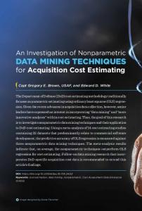
A spectrum (plural is spectra) is a graph of intensity (amount) of light emitted by an object as a  function of the wavelength of the light. Astronomers frequently measure spectra of stars, and  use these measurements to study stars. Each object has a unique spectrum, like a fingerprint is  to a person. An object's spectrum gives us information about the wavelengths of light the object  emits, its color (from peak intensity), temperature (using Stefan's law), distance from the earth  (using Hubble's law), and a hint towards its chemical composition (from the absorption and  emission lines). Thus, spectrum analysis is one of the best sources of knowledge of a celestial  object. 1.1.5 Input data used for the classification The input data will be observational and non­observational astronomy data, i.e magnitudes, and  colors,  from the various Survey catalogs. Each of the survey catalogs stores magnitudes of  different parts of the spectrum for the objects they observe. For each type of object (star, galaxy,  quasar, active galactic nuclei, etc.)  it would be possible to characterize the object based on the  range of values of the chosen parameters. In the past, before automated classification systems  were developed, astrophysicists classified the objects based on the spectrum analysis. Different  classes of objects emit different types of radiations and hence their spectra would also vary  accordingly. The factor that helped in the classification is that, objects of the same class show  certain similarities in their spectra. Thus, spectra was used for classification. Now, the data of  the surveys give us information about certain parts of the spectrum, i.e the magnitudes and  colors correspond to features in the spectrum, hence these would contain information that can  classify the objects and would be important parameters in the classification. 1.1.6 Spectra of Stars, Galaxies and Quasars The spectra of the astronomy objects would easily aid in identification of the object. Figure1.1: Spectrum of a typical star

        8/33

Subhashini(nitk)

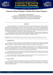
Figure1.2: Spectrum of a typical galaxy

Figure1.3: Spectrum of a typical Quasar

        9/33

Subhashini(nitk)

Chapter 2 Literature Survey Classification of astronomical objects  was one of the earliest applications  of datamining   in  astronomy. It was used in the development of an automatic star­galaxy classifier. As  newer  algorithms are being developed the classification results are also improving. The different data  mining techniques used for classification have shown varying success rates. The success of the  algorithm has also depended on the choice of the features or attributes chosen for the clustering.  An interesting aspect is that, data mining tools have also been used to identify the relevant and  significant features that help in better classification.

2.1 Review of existing systems Neural  Networks  has  proved  to  be a  powerful  tool in  extracting  necessary  information   and  interesting patterns from large amounts of data in the absence of models describing the data.  Automated   clustering   algorithms   for   classification   of   astronomical   objects   [7.6]   have   used  supervised neural networks, to be specific, Linear Vector Quantization (LVQ), Single Layer  Perceptron (SLP) and Support Vector Machines (SVM) for multi­wavelength data classification.  Their classification was based on the properties of spectra, photometry, multi­wavelength etc.  They used data from the X­ray(ROSAT), optical (USNO­A2.0) and infrared(2MASS) bands.  The parameters they chose from different bands are B − R (optical index), B + 2.5log(CR)  (optical­X­ray index), CR, HR1 (X­ray index), HR2 (X­ray index), ext, extl, J − H (infrared  index), H − Ks (infrared index), J + 2.5log(CR) (infrared­X­ray index).  For supervised methods  the input samples had to be tagged to know classes, for this they chose objects from the catalog  of AGN [ Veron Cetty & Veron, 2000].     They concluded that LVQ and SLP showed better performance when the features were fewer in  number; and SVM showed a better performance when more features were included. In   2006 with more data available about astronomy objects  from radio surveys and   Infrared  surveys,   Bayesian   Belief   Networks(BBN),   Multi­Layer   Perceptron   (MLP)   and   Alternating  Decision   Trees(ADTrees)   were   used   to   separate   quasars   and   non­quasars[7.5].   Radio   and  infrared rays are in different ends of the spectrum and can be used to better identify quasars.  The radio data was obtained from the FIRST survey and infrared data from the 2MASS. They  cross­matched the data from both surveys to obtain one­to­one entries ­to get the entire set of  radio and infrared details on the common objects­ which were again matched with the Veron­ Cetty & Veron catalog and the Tycho­2 catalog. The chosen attributes from different bands were  logF peak (F peak: peak flux density at 1.4 GHz), logF int (F int: integrated flux density at 1.4  GHz),   f   maj   (fitted   major   axis   before   deconvolution),   f   min   (fitted   minor   axis   before  deconvolution), f pa (fitted position angle before deconvolution), j − h (near infrared index), h−k  (near infrared index), k+2.5logF int, k+2.5logF peak, j+2.5logF peak, j + 2.5logF int. From the  comparison of BBNs, ADTrees and MLP methods of classification it was concluded that all the  three models achieved an accuracy between 94% and 96%. The comparison also re­established  the fact that doing feature selection, to identify relevant features, increased the accuracy in all  the three methods. Considering both accuracy and time, the ADTree algorithm proved to be the  best of the three.           10/33

Subhashini(nitk)

Based on the success of ADTree algorithm in identification of quasars, in 2007, Zhang & Zhao  used Decision Tables for classifying  point sources using the FIRST and 2MASS databases[7.4].  The features and data that they used was largely similar to what they had used for the BBN,  MLP and ADTree models. Also, point source objects (like stars and quasars) tend to have their  magnitude values falling in a particular range making the data more suitable to be classified  using decision tree like structures.  In addition to this they focussed on enhancing their feature  selection   technique,   they   used   the   Best­first   search   feature   selection.   By   using   the   optimal  features from the selection method they were able to conclude that the best­first search was  more effective than the histogram technique (used previously by Zhang & Zhao). The Decision  Table method also had a much higher accuracy (99%) in the case of quasars which proved that  this was better than the previous models (BBN, MLP and ADTree). In 2008, SDSS(Sloan Digital Sky Survey) made available the data of astronomical objects from  the visible region of the spectrum.  This provided a larger number of attributes to experiment  with.   Since   SVMs   had   shown   improved   results   (in   2004)with   more   attributes   during   the  classification of these objects, Kd­tree and Support Vector machines were used for separating  quasars from large survey databases [7.1]. Here the databases from SDSS and 2MASS catalogs  were used. The features used in order to study the distribution of stars and quasars in the multi­ dimensional space, were the different magnitudes: PSF magnitude (up, gp , rp , ip , zp  ), model  magnitude (u, g, r, i, z) and model magnitude with reddening correction ( u′, g′, r′ ,i′ ,z ′) from SDSS data, J, H and Ks magnitudes from 2MASS catalog.  This study showed that  both Kd­trees and SVMs are efficient algorithms for point source classification. It was also  observed that,  while SVM showed better  accuracy, Kd­tree required less  computation   time.  They also concluded that both the algorithms' performance was better when the features were  fewer 2.2  Problems with existing systems and suggestions for improvement 2.2.1. Most algorithms have been used to classify just 2 object classes at a time. Most algorithms have been used to classify just stars and galaxies or quasars and galaxies,  But not all three together. There might be a possibility of using the same methods to cluster  the   objects   differently,   to   characterize   objects   into   stars,   quasars,   galaxies   or   others,  provided that these objects are characterized by the same parameters and we can include  these objects in our training process.   If a single algorithm can be used to classify the  objects into a wider category, it would save an enormous amount of time as compared to  running many different algorithms on the same dataset.    2.2.2. Euclidean distance measure may not be the most suitable for astronomical objects. Astronomy data parameters are of a very different nature compared to general numerical n­ dimensional   data.   Although   each   astronomy   object   may   be   viewed   as   a   point   in   n­ dimensional space (n values for each of the attributes) it is probably not the right way to  view them since these n values give a different meaning when we look at the spectra of the  object and how the parameters define the shape of the spectra(or a crude curve). Euclidean  distance measure is the common distance measure employed by all existing algorithms.  However, by looking at the data from a different perspective it might be better to try and  identify or develop a distance measure that is more suitable for astronomy data objects.         11/33

Subhashini(nitk)

2.2.3. Feature selection Most of the algorithms do not employ a feature selection mechanism. Feature selection  mechanism is one which recognizes some parameters as more significant than others in  order   to   discriminate   between   the   type   of   objects.   An   optimum   subset   of   the   entire  parameter list would be able to perform as well as or even better than the entire set. There  can  be a reduction in the time complexity and an increase in the accuracy by performing  feature selection. Either by using methods like principal component analysis (PCA) or by  experimenting with the various attributes we can try and identify the more significant  features amongst them. 

        12/33

Subhashini(nitk)

Chapter 3  Methodology 3.1 Identify features or parameters that can aid in characterizing the classes. The survey data for each object would include all the features that have been captured. However,  all of them might not be necessary to discriminate between our chosen classes. The parameters  required   for   the   classification   are   identified   and   chosen   from   the   vast   amount   of   data.  Understanding   the   interdependencies   among   the   different   features   is   necessary   for  understanding the current models of classifications and identifying their flaws. This would also  be one of the primary objectives. An increase in the accuracy of classification and reduction in  computation time can be achieved by choosing an optimal set of significant characteristics.  Hence it would be necessary for us to identify and select relevant parameters. Stars, Quasars and Galaxies can be primarily identified from their spectrum. Hence, we choose  to   work with  photometric  parameters   for  the  classification.  Model  magnitude  values   of   the  object   at   multiple   wavelengths   would   be   ideal   attributes   for   classifying   stars,   galaxies   and  quasars since these are the values that are at different points in the spectrum. Color values (a  ratio of magnitudes at 2 different wavelengths) will also aid in the classification as these would  be better parameters for comparing the spectrum (curve­shape) of the objects. In addition to  this, the use of red­shift values will also increase the accuracy of classifying quasars from other  objects since quasars generally tend to have higher red­shifts. 3.2 Study of data mining tools that aid in classifying astronomy objects We make a detailed study of the data mining techniques that have been used to classify the  objects and identify the problems existing in them. Looking in to more recent developments, we  try to identify relevant algorithms that can be used to classify astronomical objects. We would  also make modifications to the existing algorithms and new algorithms to suit our needs. Our  aim would be to come up with a set of algorithms that would bring improvements – in terms of  accuracy or computation time ­ in the automated classification process. 3.3 Gather  data on celestial objects from the various surveys. There   a   number   of  sky  surveys   that   are   conducted   by  various   organizations   which   help   in  gathering information about the celestial sphere. Each of the surveys gather data pertaining to  different frequencies in the spectrum. e.g Chandra Telescope gathers X­ray information, SDSS  (Sloan Digital Sky Survey) gathers multi­wavelength data on 5 different bands, FIRST survey  has radio data and so on. They each use different co­ordinate systems to map the sky. In order to  classify an object into a specific class, we would need the properties of of the radiations of the  objects in all the different parts of the spectrum. We would need to correlate information from  the different surveys and build a dataset for very large number of objects. The Sloan Digital Sky Survey (SDSS) data would be able to satisfy our need for getting model  magnitude values at multiple locations spread out in the spectra of an object. The SDSS uses  five   filters   –   Ultraviolet   (u)   3543  Å(angstroms),   Green   (g)   4770   Å,   Red   (r)   6231   Å,   Near  Infrared (i) 7625 Å, and the Infrared (z) 9134 Å. The u, g, r, i and z values and the labels of the          13/33

Subhashini(nitk)

objects from SDSS database will be the five basic parameters for the classification of stars,  galaxies and quasars. From the 5 values we will also be able to derive the color values that can  help enhance the classification. In addition to the model magnitudes we also use psf magnitudes  (they are relative flux values obtained using a different function than what is used to obtain  model magnitudes) as additional attributes in order to be able to obtain a clearer classification  of galaxies. 3.4 Apply the algorithms on the chosen parameters, make improvisations. The data is divided for training and testing purposes as required by the chosen algorithms. We  can use existing softwares to test the results of some of the algorithms that have been used for  classification by other astronomers. E.g the WEKA software has been used by some of the  astronomers to classify stars and quasars using SVMs and kd­tree algorithms. Rapid Miner is  another   free   and   open   software   that   could   aid   us   in   this   regard.   We   would   then   build   an  application   based   on   the   newly   developed   algorithm   and   also   include   functions   for   the  validation of its classification. This would give us the freedom to make many small changes  with   the   algorithm   –   like   using   different   distance   measures   or   clustering   techniques   ­   and  compare the performance. 3.5 Results and conclusion The final phase is to compare the performance of our new algorithms with that of the existing  ones with respect to classification of the astronomical objects. We need to see if there has been  any improvement in the accuracy or reduction in time. We would also need to look into the  success of our algorithms in classifying the new categories of objects.

        14/33

Subhashini(nitk)

Chapter 4 Closer study of relevant data mining algorithms 4.1DBSCAN and GDBSCAN DBSCAN is a Density Based Algorithm for Discovering Clusters in Large Spatial Databses[7.7]  (Ester et al,1996). This  algorithm uses the notion of density (the number of objects present in  the neighbourhood space of a chosen object) to form clusters. This algorithm uses the following  definitions: 1.  Eps­neighborhood  of a point: The Eps­neighborhood of a point p, denoted by NEps(p), is  defined by NEps(p) = {q ∈D | dist(p,q) ≤ Eps}. 2. directly density­reachable: A point p is directly density­reachable from a point q wrt. Eps,  MinPts if   1) p ∈ NEps(q) and   2) |NEps(q)| ≥ MinPts (core point condition). 3. density­reachable: A point p is density­reachable from a point q wrt. Eps and MinPts if there  is a chain of points p1, ..., pn, p1 = q, pn = p such that pi+1 is directly density­reachable from pi. 4. density­connected: A point p is density­ connected to a point q wrt. Eps and MinPts if there  is a point 'o' such that both, p and q are density­reachable from 'o' wrt. Eps and MinPts. 5. cluster: Let D be a database of points. A cluster C wrt. Eps and MinPts is a non­empty subset  of D satisfying the following conditions:      1)  ∀  p, q: if p  ∈  C and q is density­reachable from p wrt. Eps and MinPts, then q  ∈  C.  (Maximality)    2) ∀ p, q ∈ C: p is density­connected to q wrt. EPS and MinPts. (Connectivity) The following images illustrate this: Figure4.1: DBSCAN clustering on 3 different databases

     

The basic concept used in this algorithm is to cluster those objects that are density reachable  and density connected, and it can also define objects that belonged to the border of a cluster. A  detailed description of the algorithm can be found in the book  Data Mining  Techniques by  Arun.K.Pujari(Pg.123). 

Reasons for choosing to work with DBSCAN: 1. Astronomy   objects   of   the   same   class   tend   to   have   similar   color   values   (ratio   of          15/33

Subhashini(nitk)

magnitudes are similar although the magnitude itself might be different). The use of  SVMs to classify astronomy objects using SDSS survey data has shown reasonably good  results   with   respect   to   accuracy   of   classification   [7.1].   SVMs   generate   a   separating  hyper­plane to classify objects, but based on closeness of color values, an algorithm that  can find arbitrary clusters may be able to fare better. [ i.e SVMs try to identify a plane in  n­dimensions that helps in separating the different classes of objects from the supplied  training data. Now, if the object classes can be identified by a single separating plane  then considering the fact that the astronomy data objects chosen have fairly similar range  of values, it might be possible to cluster them using a density based algorithm.] 2. DBSCAN also incorporates the concept of nearest neighbours (MinPts) which would  help cluster astronomy objects, especially quasars better since the values of magnitudes  and colors of the data object tend to fall within a small range. GDBSCAN  [7.8] , a further generalization of the DBSCAN algorithm gives greater freedom  (or multiple options) with respect to the choice of defining the neighbourhood space of an  object according to the application. This algorithm introduces the concept of adding weights to  the parameters in computing distance between objects and in defining Eps which is used for  computing the neighborhood density. GDBSCAN being a more generalized approach of the DBSCAN includes different means for  finding the density in the neighborhood space for n­dimensional data objects. The idea of giving  different weights to the parameters can be used to cluster quasars better since most quasars have  a   higher   red­shift   value   (z'),   giving   more   weight­age   to   this   factor   may   help   us   improve  classification accuracy of quasars. Advantages: 1. The space required for storing the data is less. Hence, its speed is also better. The operations  that requires most time in this algorithm is the one used for identifying the objects within the  neighborhood. By choosing appropriate Eps and MinPts, the number of times this operation  needs to be executed can be reduced. Disadvantages: 1. Choosing Eps for defining the neighborhood can be tricky. Finding the right value for Eps  that is most appropriate for the given dataset is difficult. Also, the Eps value for quasar on one  hand may be lower but stars and galaxies may require a higher value inorder to be clustered  correctly. We need to find an Eps that is optimum in clustering all our data classes. 4.2  Decision Trees A decision tree is a classification scheme which generates a tree and a set of rules, representing  the model of different classes from a given data set. The decision tree model is constructed from  the training set with the help of numerical and categorical attributes. Each node at a branch uses  the value of the attributes to to derive the rules. The leaves of the tree contain the label of the  classes. When the test data is input , the tree is traversed from the root and the branch chosen  depends on the parameters under consideration in that node. Finally the test input is assigned  the class of the leaf node it reaches after traversing a  particular path of nodes from the root to          16/33

Subhashini(nitk)

that leaf. Details about determining the splitting attribute and splitting criteria are referred from  [7.9]( pp 154­195). The values for the magnitudes and colors of astronomy objects tend to fall within a close range.  [The average range into which each parameter falls can be found from the training sample].  Based on this fact, it may be possible to form rules to group the objects [like, objects having  z>=A, u­g > B and i­z