Algorithms for Rendering Depth of Field Effects in Computer Graphics Brian A. Barsky1,2 and Todd J. Kosloff1 1 Computer Science Division 2 School of Optometry University of California, Berkeley Berkeley, California 94720-1776 USA
[email protected] [email protected] http://www.cs.berkeley.edu/~barsky Abstract: Computer generated images by default render the entire scene in perfect focus. Both camera optics and the human visual system have limited depth of field, due to the finite aperture or pupil of the optical system. For more realistic computer graphics as well as to enable artistic control over what is and what is not in focus, it is desirable to add depth of field blurring. Starting with the work of Potmesil and Chakravarty[33][34], there have been numerous approaches to adding depth of field effects to computer graphics. Published work in depth of field for computer graphics has been previously surveyed by Barsky [2][3]. Later, interactive depth of field techniques were surveyed by Demers [12]. Subsequent to these surveys, however, there have been important developments. This paper surveys depth of field approaches in computer graphics, from its introduction to the current state of the art. Keywords: - depth of field, blur, postprocess, distributed ray tracing, lens, focus, light field.
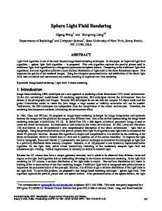
Figure 1: (left) Image before and after depth of field has been added via postprocessing (courtesy of Indranil Chakravarty [33]). (right) A dragon scene rendered with a distributed ray tracing approach (courtesy of Magnus Strengert [23]).
1 Introduction Computer generated images by default render the entire scene in perfect focus. Both camera optics and the human visual system have limited depth of field, due to the finite aperture or pupil of the optical system. For more realistic computer graphics as well as to enable artistic control over what is and what is not in focus, it is desirable to add depth of field blurring. Starting with the work of Potmesil and Chakravarty[33][34], there have been numerous approaches to adding depth of field effects to
computer graphics. Published work in depth of field for computer graphics has been previously surveyed by Barsky [2][3]. Later, interactive depth of field techniques were surveyed by Demers [12]. Subsequent to these surveys, however, there have been important developments. This paper surveys approaches to depth of field approaches in computer graphics, from its introduction to the current state of the art.
2 Optics An image is formed in an optical system when light enters, is refracted by the lens, and impinges on the image capture device (which may be film, a digital sensor, or a retina). To capture adequate light to form an image, the optical system must include an aperture of sufficient size. The light originating from a given point in the scene thus converges at only one depth behind the lens, and this depth is not necessarily that of the sensor (Figure 2). Therefore images have limited depth of field; that is, objects that are not sufficiently near the focus depth will appear blurred. Points on objects at a given depth will appear spread over a region in the image known as the circle of confusion (CoC). To see how to compute the size of the diameter of the CoC using a thin lens model, the reader is referred to Barsky [2]. A thorough treatment of optics can be found in [8]. Computer graphics methods for rendering 3D scenes typically use a pinhole camera model, leading to rendering the entire scene in perfect focus. Extra effort is required to simulate limited depth of field and an aperture that has a finite size.
Object space methods can be further subdivided into those based on geometric optics, and those based on wave optics. Most work in computer graphics uses geometric optics, which is sufficiently accurate for many purposes. However, diffraction and interference do play a role in the appearance of defocused images. Wave-propagation approaches have therefore been investigated, as a very direct way to simulate such effects. Image space methods can be further subdivided into methods primarily suitable for computer generated images, and those applicable to computational photography. Traditional postprocess methods require an accurate depth map to know where and how much to blur, but such a depth map is difficult to acquire for a real-world photograph. Light fields, on the other hand, allow digital refocusing, without the need for a depth map. Light fields require specialized equipment to capture as well as substantial storage, but the algorithms involved are straightforward, produce good images, and can represent scenes of arbitrary complexity.
4 Object-Space Approaches 4.1 Distributed ray tracing
Figure 2: A point in the scene (left) images as a disc on the image plane (right), leading to depth of field effects (image courtesy of Pat Hanrahan [25]).
3 Overview We can categorize depth of field methods in computer graphics in several ways. First, we can differentiate between object space and image space methods. Object space methods operate on a 3D scene representation, and build depth of field effects directly into the rendering pipeline. Image space methods, also known as postprocess methods, operate on images that were rendered with everything in perfect focus. The images are blurred with the aid of a depth map. The depth map is used along with a camera model to determine how blurred each pixel should be. In general, object space methods generate more realistic results and suffer fewer artifacts than image space methods. However, image space methods are much faster.
Geometric optics can be directly simulated by distributed ray tracing [11]. Rather than tracing one ray per pixel, which simulates a pinhole camera, several rays are traced per pixel, to sample a finite aperture. For a given pixel, each ray originates at the same point on the image plane, but is directed towards a different point on the lens. Each ray is refracted by the lens, and then enters the scene. Since distributed ray tracing accurately simulates the way an image is actually formed (ignoring wave effects), images generated this way appear quite realistic, and they serve as the “gold standard” by which we can evaluate postprocess methods. Unfortunately, a great many rays per pixel are required for large blurs, making distributed ray tracing a very time consuming process. When insufficiently many rays are used, the images contain artifacts in the form of noise. Images with depth of field generated by distributed ray tracing are shown in Figure 1 (right) and Figure 4.
4.2 Realistic camera models Cook originally used distributed ray tracing with a thin lens camera model, and Kolb et al. [25] later extended this method to model specific real-world lenses. First, lens specifications are obtained from the manufacturer of the lens that is to be simulated. Often, camera lenses take the form of a series of
spherical lenses with various radii, interspersed with stops (Figure 3). Next, the exit pupil is determined, as this determines the disc on the back of the lens that must be sampled. Finally, distributed ray tracing is performed by tracing rays from points on the image plane to points on the exit pupil. These rays are refracted by each lens of the assembly before entering the scene. This process accurately takes into account both the depth of field properties of the lens as well as the perspective projection, including distortions. Examples can be seen in Figure 4.
Figure 3: An assembly of lenses, as found in a typical camera (image courtesy of Pat Hanrahan [25]).
4.3 Accumulation Buffer It is possible to use the accumulation buffer [17] found on standard rasterization hardware to render depth of field effects by sampling the aperture. A collection of pinhole-based images is rendered, and the accumulation buffer is used to average those images. Each pinhole-based image is rendered with a slightly different projection matrix that places the pinhole at a different location on the aperture. In principle, this method is very similar to distributed ray tracing insofar as many samples per pixel are taken and averaged. However, the accumulation buffer method is faster because rasterization hardware is quite fast compared to ray tracing. Distributed ray tracing, however, enables adaptive control over the number and distribution of samples per pixel, leading to higher accuracy with fewer rays, compared to uniform sampling. But the accumulation buffer must render an entire pinhole-based image at a time, because rasterization hardware is optimized for rendering entire images, rather than individual pixels. The accumulation buffer method must thus use the same number and distribution of samples for each pixel.
4.4
Wave-Propagation Methods
Both distributed ray tracing and the accumulation buffer assume geometric optics, meaning that diffraction and interference are ignored. If we treat our scene as a large collection of point light sources, each emitting a wave front of appropriate wavelength, the propagation of these wave fronts can be tracked through space [42][43]. An image plane is placed at a particular location, and the contributions from all the wave fronts are summed, then the amplitude is taken to determine pixel values. This process is generally carried out in the frequency domain, so that Fast Fourier Transforms [14] can provide a speedup. As this method directly simulates light waves, diffraction and interference are automatically included.
4.5
Figure 4: Three different lens assemblies, and the resulting images. Notice the barrel distortion in the top image, and notice the effect of varying focal length in the middle and bottom image. (Images courtesy of Pat Hanrahan [25].)
Splatting
When the amount of detail in a scene is sufficiently high, it sometimes makes sense to describe the scene not as a collection of geometric primitives with texture maps, but rather as a dense collection of point samples. A standard way to render point-based scenes is elliptical weighted average splatting [44], which renders each point as an elliptical Gaussian. The point samples are stored in a tree, and points are drawn from appropriate levels of the tree to achieve automatic level of detail.
Although DoF effects in point based scenes could be rendered using the accumulation buffer, it is more efficient instead to modify the splatting method, as Krivanek et al. showed in [24]. Each point sample is convolved with the appropriate PSF, before splatting. In the case of a Gaussian PSF, the result is simply to increase the standard deviation of the Gaussian splat. Therefore, DoF blurring fits naturally into the splatting pipeline. A resulting image can be seen in Figure 5. This method is accelerated by drawing from coarser levels of the point sample tree, when the blur is large (Figure 6). The method is faster due to fewer points being rendered, but it still maintains accuracy because the lost detail would have been blurred anyway.
ought to be blurred. This method has the advantage of generating precise, noise-free images, in constrast to sampling methods such as distributed ray tracing and the accumulation buffer, which can suffer from noise or ghosting even when very large numbers of samples are used.
5 Image-Space Approaches The ideal post-process method would satisfy all of the following criteria:
Choice of point spread function The appearance of blur can be defined by considering the point spread function (PSF), which shows how a single point of light appears after having been blurred. Since different optical systems have different PSFs, a good DoF postprocess method should allow for the use of a wide variety of PSFs.
Per-pixel blur level control
Figure 5: A complex point-sampled object with depth of field (image courtesy of Jaroslav Krivanek [24]).
At each pixel, the amount of blur depends on depth. Since objects can have complex shape, each pixel can have a different depth and hence a different amount of blur. Some postprocess methods use pyramids or Fourier transforms, which operate at specific blur levels over entire images. Ideally, however, a postprocess method should have complete per-pixel control over the amount of blur.
Lack of intensity leakage A blurred background will never blur on top of an infocus foreground in a real image. However, this property is not respected by the simple linear filters sometimes used for DoF postprocessing. Therefore such methods suffer from intensity leakage artifacts, which detract from the realism of the resulting images.
Figure 6: (left) Point-sampled chessboard, rendered using splatting. (right) Illustration of the decreased point density used in highly blurred regions (image courtesy of Jaroslav Krivanek [24]). 4.6 Analytical Visibility Catmull describes an analytical hidden surface removal algorithm for rendering polygonal scenes, based on clipping polygons against one another [10]. Catmull solves the aliasing problem analytically as well, by integrating the visible polygons across the entire width of each pixel. Given this framework, he shows how it is straightforward to add depth of field effects (or motion blur) simply by increasing the width of the anti aliasing filter for polygons that
Lack of depth discontinuity artifacts In real images, the silhouette of a blurred foreground object will be soft, even if the background is in focus. Unfortunately, in this case, simple linear filters sometimes lead to the blurred object having a sharp silhouette. This artifact occurs where the depth map of an image changes abruptly, so we refer to this as a depth discontinuity artifact.
Proper simulation of partial occlusion In real images, blurred foreground objects have soft edges at which some portions of the background are visible. We refer to this as partial occlusion, since the background is only partially blocked by the foreground. These visible parts of the background would not be visible in the case of a pinhole image of
the same scene. The geometry of partial occlusion is illustrated in Figure 5. Since a postprocess method starts with a single pinhole image as input, it is difficult in this case to correctly simulate partial occlusion. Generally, background colors must be interpolated from the colors that are known.
Figure 5: Partial Occlusion (image from Barsky [2]).
High performance Directly filtering an image in the spatial domain has a cost proportional to the area of the PSF. For large PSFs, the blurring process can take several minutes. Ideally we would like interactive or real time performance, motivating some of the more recent work in the field. No post-process method satisfies all these criteria; a full solution is still an open problem at this time.
5.1 Linear Filtering Potmesil and Chakravarty described the first method for adding depth of field to computer generated images [33][33]. Their method is a postprocess method, using a spatially variant linear filter and a depth-dependent PSF. Their filter operates directly in the spatial domain, and thus has a cost proportional to the area of the PSFs being used. The linear filter can be expressed by the following formula:
B( x, y) psf ( x, y, i, j ) S (i, j ) i
j
where B is the blurred image, psf is the filter kernel, which depends on the point spread function, x and y are coordinates in the blurred image, S is the input (sharp) image, and i and j are coordinates in the input image. Results from this method are shown in Figure 6. Potmesil and Chakravarty used PSFs derived from physical optics, incorporating diffraction off the edge of the aperture, and interference on the image plane. This method did not attempt to mitigate intensity leakage or depth discontinuity artifacts.
Figure 6: Image blurred using a linear filtering approach, with the focus at different depths (images courtesy of Indranil Chakravarty [33]).
5.2 Ray Distribution Buffer Shinya proposed a replacement for the previous linear filtering method that explicitly handles visibility, thereby eliminating intensity leakage [39]. Rather than directly create a blurred image, Shinya first creates a ray distribution buffer, or RDB, for each pixel. The RDB contains one z-buffered entry for each of several discretized positions on the lens from which light can arrive. By decomposing each pixel in this way, complex visibility relationships can be easily handled via the z-buffer. After the RDBs have been created, the elements of each RDB are averaged to produce the blurred pixel color. The RDB method handles visibility quite well, at the cost of additional time and memory compared to a straightforward linear filter. It is interesting to note that the set of RDBs constitute the camera-lens light field of the scene. Light fields and their connection to DoF will be discussed later in this paper.
5.3 Layered Depth of Field Scofield shows how Fast Fourier Transforms can be used to efficiently perform depth of field postprocessing for the special case of layered planar, screen-aligned objects [38]. Each layer is blurred by
a different amount, using frequency domain convolution. Then, the blurred layers are composited with alpha blending [32]. The FFT allows any point spread function to be efficiently used, and there is no additional cost for using large PSFs. The use of layers and alpha blending provides a good simulation of partial occlusion, and completely eliminates intensity leakage. Scofield's method is simple to implement, but the FFT convolution requires that each layer have only a single level of blur. Thus, there can be no depth variation within a layer.
5.4 Occlusion and Discretization The restriction to planar, screen-aligned layers is severe. This is addressed by the method described in Barsky [4][6] where objects are made to span layers, even though each layer is blurred using a single convolution. First, layers are placed at various depths. The layers are placed uniformly in diopters, because the appearance of blur is linear in diopters. Next, each pixel from the input image is placed in the layer whose depth is nearest to that pixel’s depth. If each layer were simply blurred and composited as-is, then the resulting image would suffer from discretization artifacts, in the form of black or transparent bands where one layer transitions into another (Figure 7, top). This method solves this using object identification. Entire objects are found, using either edge detection or an adjacent pixel difference technique. Wherever part of an object appears in a layer, the layer is extended to include the entire object, thus eliminating the discretization artifacts (Figure 7, bottom). Another concern addressed by this method is partial occlusion. The input is a single image, so when a foreground object is blurred, no information is available as to the colors of disoccluded background pixels. This method mitigates this problem by extending background layers to approximate the missing information, using a carefully chosen Gaussian kernel.
Figure 7: Pixar’s tin-toy scene blurred by Barsky’s discrete depth method. Black bands occur at layer boundaries (top) unless object identification is utilized (bottom) (images from Barsky [4]).
characteristics of the eyes of a particular person. A wavefront measurement is taken from a human subject, and that wavefront is then sampled to create a set of PSFs, corresponding to different depths. This set of PSFs is then used with the layered scheme described in the previous section, where the PSFs are convolved with the layers and composited. An example is shown in Figure 8.
5.5 Vision Realistic Rendering Most depth of field methods attempt to simulate either a generic thin lens camera model or particular camera lenses, as is the case of Kolb et al. [25]. However, the optics of the human eye are more difficult to simulate because the cornea and lens of the eye cannot be adequately described as a small set of spherical lens elements in the way that cameras can. In vision realistic rendering, proposed in Barsky [5], data from a wavefront aberrometer instrument is used to perform depth of field postprocessing such that the blur corresponds directly to the optical
Figure 8: Vision realistic rendering. This image was generated using wavefront data from a patient with kerataconus (image from Barsky [5]).
5.6 Importance Ordering Fearing showed that the performance of depth of field rendering can be improved by exploiting temporal coherence [13]. The pixels are ranked according to an importance ordering. Pixels that have not changed significantly from the previous frame have low importance, whereas pixels that are completely different have a high importance. For the new image, DoF is applied to the more important pixels first. The processing can be interrupted early, and the time spent will have been spent primarily on the most important pixels. Therefore, a reasonable approximation is obtained in the limited time allotted.
5.7 Perceptual Hybrid Method Mulder and van Lier observe that, due to perceptual considerations, the center of an image is more important than the periphery [29]. Exploiting this observation, they create a hybrid depth of field postprocess method that is accurate and slow at the center, but approximate and fast at the periphery. For the fast approximation, they create a Gaussian pyramid from the input image, pick a level based on the desired amount of blur, and up sample that level by pushing it through the pyramid. The fast approximation results in a blurred image that suffers from some degree of blocky artifacts. The periphery is blurred in a more direct and slow, but higher quality fashion using circular PSFs.
5.8 Repeated Convolution Rokita aimed to improve the speed of depth of field postprocessing such that it would be suitable for interactive applications such as virtual reality. This approach uses graphics hardware that can efficiently convolve an image with a 3x3 kernel [35]. Large blurs can be achieved by using this hardware to repeatedly execute 3x3 convolutions. Although this method is faster than direct filtering, it becomes slower as blur size increases and the PSF is restricted to be a Gaussian.
5.9 Depth of Field on the GPU Scheueremann and Tatarchuk developed a DoF method implemented as a GPU pixel shader that runs at interactive rates and largely mitigates intensity leakage [36][37]. For each pixel, the size of the CoC is determined using an approximation to the thin lens model. Next, Poisson-distributed samples are taken within the circle of confusion, and averaged. For a large CoC, a great many samples would be needed to eliminate noise. To avoid this, a 1/16th scaled down sampled version of the image is used when sampling a large CoC. In this manner, fewer samples are
needed since a single pixel in the down sampled image represents numerous pixels in the input image. To reduce intensity leakage, sample depths are compared to the depth of the pixel at the center of the CoC. If the sample lies behind the center pixel, then that sample is discarded. Unfortunately, depth discontinuity artifacts are not addressed in this method.
5.10 Summed Area Table Method As an alternative to sampling the CoC, the average over a region of the image can be computed using a summed area table [16]. The SAT has the advantage that a fixed (small) amount of computation is required, no matter how large the blur, and there is no need to distribute sample points or create a down sampled image. The SAT was originally developed for anti-aliasing texture maps. However, Hensley showed how the SAT can be used for depth of field postprocessing [20] and furthermore that this method can be accelerated by a GPU, using a recursive doubling technique to generate a new SAT for every frame. Unfortunately, the SAT method does not address the intensity leakage or depth discontinuity issues.
5.11 Pyramidal Method Kraus and Strengert show how to combine a carefully constructed GPU-enabled pyramidal blur method with a layering approach somewhat similar to Barsky [5], to achieve real time DoF postprocessing while eliminating many instances of intensity leakage and depth discontinuity artifacts [24]. First, the scene is distributed into layers, based on depth. Rather than binning each pixel entirely into the nearest layer, pixels are distributed proportionally to several adjacent layers, according to a carefully chosen distribution function. This proportional distribution serves to mitigate discretization artifacts at the layer boundaries. Second, background pixels, which may become disoccluded, are interpolated, also using a pyramid method. Next, each layer is blurred by down sampling to an appropriate pyramid level, and up sampling. The weights used during the up sampling and down sampling are carefully controlled to reduce the block artifacts that occur with simpler pyramid methods. Finally, the blurred layers are composited using alpha-blending. An example is shown in Figure 9. This method is faster than previous layer-based methods based on FFTs but is only applicable to the limited class of PSFs to which pyramids can efficiently apply.
5.14 Generalized and Semantic DoF
Figure 9: A dragon scene blurred using pyramidal methods on the GPU (image courtesy of Magnus Strengert [23]).
5.12 Separable Blur Just as blur can be applied efficiently for Gaussianlike PSFs using pyramids or for rectangular regions using SATs, separable PSFs can also be applied efficiently. Zhou showed how a separable blur can be used for depth of field postprocessing, with elimination of intensity leakage [41]. The method is simple to describe and implement: First the rows of the image are blurred. Then, the columns of the resulting image are blurred. Separable blur has a cost proportional to the diameter of the PSF; this is a significant improvement over direct filtering which has a cost proportional to the area of the PSF. Zhou also shows how to eliminate intensity leakage by appropriately ignoring pixels while blurring the rows and columns. The entire method is implemented on a GPU, and runs at interactive rates for moderate PSF sizes.
Most methods for simulating depth of field naturally aim to accurately simulate real-world optics. However, depth of field is also an artistic tool, not merely an artifact of the image formation process. As an artistic tool in computer graphics, we do not necessarily have to be limited by the types of lenses we know how to build. Specifically, it may be desirable to have regions in focus that have unusual shape, such as spheres or cylinders, while blurring everything else. Alternatively, we may wish to select a handful of discontiguous people from a crowd, by focusing on them and blurring the others. Kosara refers to this usage of blur as semantic depth of field, and presented the first work describing how it might be implemented by blurring each object independent of the others [26]. The authors [27] later showed how to use simulated heat diffusion to provide more finegrained control, allowing the blur amount to be a continuously varying field located within the space of the scene. Figure 10 shows an example of generalized depth of field.
5.13 Approaches Based on Simulated Heat Diffusion Heat diffusion is a natural physical process that exhibits blurring despite being unrelated to optics. Specifically, if a thermally conductive object has an uneven distribution of heat, then that distribution will progressively become more even, or blurred, over time. The differential equations of heat diffusion [9] provide an alternative mathematical framework from which to derive blurring algorithms. We consider an image as a conductive surface, with intensity variation encoded as heat variation. Bertalmio et al. [7] showed how simulation of heat diffusion on a GPU could be used to simulate depth of field effects in real time for moderate blur sizes. Kass et al. [22] showed that plausible depth of field postprocessing can be achieved in real time, even for arbitrarily large sized blurs, by using the alternating directions implicit method to solve the heat equations.
Figure 10. Generalized depth of field. A plus-sign shaped region is in focus (image from Kosloff and Barsky [27]).
5.15 Light Fields 5.15.1 Introduction to Light Fields Light fields [28] and lumigraphs [15] were originally introduced as a means for capturing and representing the appearance of a scene from many different points of view, so that the scene can later be viewed at interactive rates, regardless of the complexity of the scene. The two-plane parameterization is a standard way to encode light fields, and is particularly relevant to depth of field. To represent a light field using this parameterization, two parallel planes are first arbitrarily chosen. A ray can be described by giving a point on each plane; the ray is along the line
connecting those two points. If we assume that radiance does not change along a ray, then we can associate one color with each ray, thereby encoding the light field as a four-dimensional data set. There exists an inherent light field within ordinary cameras, which has a natural two-plane parameterization. We consider light that enters the lens, and impinges on the film/sensor plane of the camera. Each light ray can be described by specifying where the ray entered on the lens and where it stopped on the film/sensor, and this engenders the two-plane parameterization. A typical camera effectively sums all the light hitting a given point on the film/sensor, no matter from which part of the lens it emanates. Therefore, if we have a film/sensor-lens light field, we can perform an integration step to create an image with DoF effects. Given a light field, we can go further, and either decrease the aperture size, or even change the location of the focus plane, during the integration step [31]. Decreasing the aperture size is a simple matter of decreasing the range of lens coordinates over which we integrate. Changing the focus plane can be performed directly, by treating the light field as a set of rays, moving the location of the film plane, and then integrating, in the style of distributed ray tracing. Alternatively, refocusing can be performed more efficiently in the frequency domain, using 4D FFTs, as shown in Ng [31]. Isaksen [21] showed how we can extend the focus plane into a focus surface by dynamically reparameterizing a light field such that a variety of different depths can be in focus in a single image.
5.15.2 Realistic Camera Models with Light Fields Light fields can be easily acquired for computer generated scenes by repeatedly rendering the scene from different points of view. Rasterization hardware can be used to accomplish this rendering efficiently. Heidrich showed how the effects of different types of lenses can be achieved by manipulating such a light field [19]. Distortion, for example, can be accurately simulated by distorting 2D slices of the light field appropriately. This image-based approach achieves lens effects similar to those that were done using raytracing in Kolb et al. [25], but this approach does so more efficiently due to the use of rasterization hardware.
5.15.3 Light-Field Camera Ng et al. built a camera that captures the lensfilm/sensor light field in a single photographic exposure [30]. An array of micro-lenses is placed in front of the film/sensor, to separate the light arriving from different directions. The light that would be summed together at a single point on the film/sensor in a normal camera is instead spread out to different locations on the film. Thus, the camera directly captures a light field. This light field can be used after the exposure has been taken to refocus and to change the aperture size. Ng et al. also analyze the captured light field to determine theoretically how much information is being captured.
5.15.4 Dappled Photography Ng's camera requires a micro-lens array, and the resulting light field suffers from low resolution. Although the underlying sensor in the camera may capture images of high resolution, much of that resolution is used to store directional samples. Higher resolution sensors may resolve this problem. Veeraghavan et al. describe dappled photography as an alternative way of capturing a light field in a single photographic exposure that mitigates the aforementioned limitations [40]. Rather than adding an array of micro-lenses, a semi-transparent mask is placed in the camera, and used to modulate the incoming light according to a known pattern. By rearranging the resulting image and taking an inverse Fourier transform, the light field can be recovered. Additionally, the modulation can be removed, resulting in a full-resolution image.
5.15.5 Defocus Magnification It is desirable to manipulate the depth of field in an ordinary photograph, in cases where no light field is available. This is a challenging task, as photographs do not typically have a depth map. Bae and Durand [1] show how we can increase the amount of blur in a photograph, for cases where the out-of-focus regions are insufficiently blurred. Rather than recovering depth, this method estimates the amount of blur at each pixel in the photograph. The amount of blur already present is used as a guide for determining how much blur to add. Since it is not possible to determine the amount of blur in regions without texture, Bae and Durand calculate blur at edges in the image, and then propagate this information into the rest of the image. An example of the defocus magnification process is shown in Figure 11.
6 Conclusion In this paper, we described a variety of methods for adding and manipulating depth of field effects for computer generated images and computational photography. Some of these methods operate in object space, and are modifications to the underlying rendering process. Others are postprocess methods, operating on images or light fields, adding or manipulating depth of field after the images have been created. We also described the challenging issues and artifacts with which depth of field postprocess methods must contend. At this time, there still does not exist any method for rendering photographic quality depth of field effects in real time, so this remains an important area of future work. Furthermore, a great deal of additional work remains to be done in computer vision, so that high quality depth maps can be reliably constructed from photographs, to enable depth of field postprocessing on existing photographs. Figure 11. Defocus magnification. Top: Original photograph. Bottom: The defocus has been magnified. Notice how the background of the bottom image is more blurred than in the top image (courtesy of Fredo Durand [1]).
5.16
Automatically Setting the Focus Depth
One application for computer generated DoF is to improve the realism of virtual reality walkthroughs and video games. To use DoF for this purpose requires a way to determine where the focus plane should be. Hillaire et al. [18] describe a method for doing so, similar in principle to the autofocus found on modern cameras. Using the idea that the objects that should be in focus are in the center, a rectangular region is placed at the center of the image. A single depth, at which to set the focus, is computed as a weighted average of the depths of all the pixels within that central region, where the weight for each pixel is the product of a spatial weight based on a Gaussian centered at the center of the image and a semantic weight function which applies greater weights to objects that are considered important. That way, important pixels will be focused on even if they represent only a small fraction of the pixels. Hillaire goes on to describe how the focus depth can be slowly varied over time, using a low pass filter, to approximate the way that the human eye undergoes accommodation. Furthermore, Hillaire presents a user study to validate the notion that adding depth of field to an interactive environment is worthwhile.
References: [1] Bae, Soonmin, Durand, Fredo. Defocus Magnification. Computer Graphics Forum. V. 26, I.3. (Proc. of Eurographics 2007). 2007. [2] Barsky, Brian A., Horn, Daniel R., Klein, Stanley A., Pang, Jeffrey A., Yu, Meng.: Camera models and optical systems used in computer graphics: Part ii, image based techniques. In: Proceedings of the 2003 International Conference on Computational Science and its Applications (ICCSA’03). pp 256–265. 2003. [3] Barsky, Brian A., Horn, Daniel R., Klein, Stanley .A., Pang, Jeffrey A., Yu, Meng: Camera models and optical systems used in computer graphics: Part i, object based techniques. In: Proceedings of the 2003 International Conference on Computational Science and its Applications (ICCSA’03). pp. 246–255. 2003. [4] Barsky, Brian A., Tobias, Michael J., Horn, Daniel R., Chu, Derrick P.: Investigating occlusion and discretization problems in image space blurring techniques. In: First International Conference on Vision, Video, and Graphics. pp. 97–102. 2003. [5] Barsky, Brian A.: Vision-realistic rendering: simulation of the scanned foveal image from wave-front data of human subjects. In: Proceedings of the 1st Symposium on Applied perception in graphics and visualization, ACM, pp. 73–81. 2004. [6] Barsky, Brian A., Tobias, Michael J., Chu, Derrick P., Horn, Daniel R.: Elimination of artifacts due to occlusion and discretization problems in image space blurring techniques. Graphical Models 67(6) pp. 584–599. 2005. [7] Bertalmio, Marcelo, Fort, Pere, SanchezCrespo, Daniel: Real-time, accurate depth of field using anisotropic diffusion and programmable graphics cards. In: IEEE
Second International Symposium on 3DPVT, IEEE (2004) [8] Born, Max, Wolf, Emil. Principles of Optics. Cambridge University Press. 1980. [9] Carslaw, H.S. Jeager, J.C. Conduction of Heat In Solids, 2nd edition. Oxford University Press.1959. [10] Catmull, Edwin. An analytic visible surface algorithm for independent pixel processing, SIGGRAPH 1984 Conference Proceedings, pp. 109-115, 1984. [11] Cook, Robert L., Porter, Thomas, Carpenter, Loren.: Distributed ray tracing. In: ACM SIGGRAPH 1984 Conference Proceedings, ACM pp. 137–145. 1984. [12] Demers, Joe. Depth of field: A survey of techniques. In: GPU Gems. pp. 375–390. 2004. [13] Fearing, Paul Importance Ordering for RealTime Depth of Field Proceedings of the Third International Computer Science Conference on Image Analysis Applications and Computer Graphics, Springer-Verlag Lecture Notes in Computer Science; Vol. 1024, pp 372-380, 1995. [14] Frigo, Matteo, Johnson, Steven. The Design and Implementation of FFTW3 Proceedings of the IEEE 93 (2) Special Issue on Program Generation, Optimization, and Platform Adaptation, pp 216-231, 2005. [15] Gortler, Steven, Grzeszczuk, Radek. Szeliski, Richard, Cohen, Michael. The lumigraph. SIGGRAPH 1996, pp 43-54. 1996. [16] Crow, Frank C. Summed-Area Tables for Texture-Mapping. SIGGRAPH 1984 Conference Proceedings, pp. 207-212, 1984. [17] Haeberli, Paul, Akeley, Kurt.: The accumulation buffer: hardware support for high-quality rendering. In: ACM SIGGRAPH 1990 Conference Proceedings, ACM (1990) 309–318. [18] Hillaire, Sebastien., Lecuyer, Anatole. Cozot, Remi., Casiez, Gery. Depth-of-Field Blur Effects for First-Person Navigation in Virtual Enviornments. Proceedings of VRST 2007. 2007. [19] Heidrich, Wolfgang. Slusallek, Philipp, Seidel, Hans-Peter. An image-based model for realistic lens systems in interactive computer graphics. Graphics Interface 1997, pp. 68-75. 1997. [20] Hensley,Justin, Scheueremann, Thorsten, Coombe, Greg, Singh Montek, Lastra, Anselmo: Fast Summed-Area Table Generation and its Applications Proceedings of Eurographics 2005. [21] Isaksen, Aaron., McMillan, Leonard. and Gortler, Steven J. Dynamically reparameterized light fields. SIGGRAPH 2000. 2000 [22] Kass, Michael, Aaron Lefohn, and John Owens. Interactive Depth of Field Using Simulated Diffusion on a GPU. Technical report. Pixar Animation Studios. 2006. Available online at http://graphics.pixar.com/DepthOfField/paper .pdf. [23] Kraus, Martin, and Strengert, Magnus. Depth of Field Rendering by Pyramidal
Image Processing, Computer Graphics Forum, 26(3), Euographics 2007. [24] Krivanek, Jaroslav, Zara, Jiri, Bouatouch, Kad.: Fast depth of field rendering with surface splatting. In: Computer Graphics International 2003. 2003 [25] Kolb, Craig, Mitchell, Don, Hanrahan, Pat: A realistic camera model for computer graphics. In: ACM SIGGRAPH 1995 Conference Proceedings, ACM, pp. 317– 324. 1995. [26] Kosara, Robert, Miksch, Silvia, Hauser, Helwig, Schrammel, Johann, Giller, Verena, Tscheligi, Manfred. Useful Properties of Semantic Depth of Field for Better F+C Visualization Proceedings of the 4th Joint IEEE TCVG - EUROGRAPHICS Symposium on Visualization (VisSym 2002), May 27-29, 2002, in Barcelona, Spain, pp. 205-210. 2002. [27] Kosloff, Todd J., Barsky, Brian A.: An Algorithm for Rendering Generalized Depth of Field Effects Based On Simulated Heat Diffusion. Technical Report No. UCB/EECS2007-19. Available online at http://www.eecs.berkeley.edu/Pubs/TechRpts /2007/EECS-2007-19.pdf. 2007. [28] Levoy, Marc., Hanrahan, Pat. Light field rendering. SIGGRAPH 1996, pp 31-42. 1996. [29] Mulder, Jurriaan D., van Lier, Robert: Fast Perception-Based Depth of Field Rendering. Proceedings of the ACM symposium on Virtual reality software and technology, pp. 129-133, 2000. [30] Ng, Ren, Levoy, Marc. Bredif, Mathieu. Duval, Gene. Horowitz, Mark. Hanrahan, Pat. Light Field Photography With a HandHeld Plenoptic Camera. Stanford Tech Report CTSR 2005-02. 2005. [31] Ng, Ren, Fourier Slice Photography. In Proceedings of SIGGRAPH 2005 2005.. [32] Porter, Thomas, Duff, Tom. Compositing digital images. In: ACM SIGGRAPH 1984 Conference Proceedings. 253–259. 1984 [33] Potmesil, Michael, and Indranil Chakravarty. A Lens and Aperture Camera Model for Synthetic Image Generation. In Proceedings of the 8th Annual Conference on Computer Graphics and Interactive Techniques, pp. 297–305. 1981. [34] Potmesil, Michael, Chakravarty, Indranil: Synthetic image generation with a lens and aperture camera model. ACM Transactions on Graphics 1(2), 85–108. 1982. [35] Rokita, Przemyslaw: Generating depth of field effects in virtual reality applications. IEEE Computer Graphics and Applications 16(2) 18–21. 1996. [36] Scheueremann, Thorsten. Advanced Depth of Field. Presentation at Game Developer Conference 2004. [37] Scheueremann, Thorsten. and Tatarchuk, Natalya. Advanced Depth of Field Rendering. ShaderX3: Advanced Rendering with DirectX and OpenGL. Charles River Media, Cambridge, MA. 2004. [38] Scofield, Cary.: 2 1/2-d depth of field simulation for computer animation. In: Graphics Gems III, Morgan Kaufmann 1994.
[39] Shinya, Mikio.: Post-filtering for depth of field simulation with ray distribution buffer. In:Proceedings of Graphics Interface ’94, Canadian Information Processing Society (1994) 59–66 [40] Veeraghavan, Ashok, Raskar, Ramesh. Agrawal, Amit, Mohan, Ankit, Tumblin, Jack. Dappled Photography: Mask Enhanced Cameras for Hetereodyned Light Fields and Coded Aperture Refocusing. ACM SIGGRAPH 2007. 2007. [41] Zhou, Tianshu, Chen, Jim X., Pullen, Mark. Accurate Depth of Field Simulation in Real Time, In Computer Graphics Forum 26(1), pp 15-23. 2007. [42] Ziegler, Remo., Croci, Simone, Gross, Markus. Lighting and Occlusion in a WaveBased Framework Eurographics 2008. [43] Ziegler, Remo., Kaufmann, Peter., Gross, Markus. A Framework for Holographic Scene Representation and Image Synthesis IEEE TVCG 2007. [44] Zwicker, Matthias., Pfister, Hanspeter., van Baar, Jeroen, Gross, Markus. EWA splatting. IEEE Transactions on Visualization and Computer Graphics. Vol (8). I(3). pp 223238. 2002.