data processing and quality control - whycos

CHAPTER 9

DATA PROCESSING AND QUALITY CONTROL

9.1

GENERAL

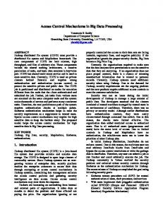
Quality assurance programmes, such as the ISO 9000 series (see ISO, 2000), have been adopted by many agencies, putting in place practices that aim to formalize and standardize procedures, from data collection, through processing, to extensive data checking. Quality assurance typically encompasses training, best practices, recording errors and malfunctions, corrective action, checking and other quality control, and independent audit of the entire operation. This chapter will cover quality control, considered here as the process of checking and validation of the data, but not the wider topic of quality assurance. Following their capture on some medium, whether paper, punched-tape or electronic digital form, hydrological data are converted to a form suitable for archiving and retrieval. In addition, at various stages, data undergo a range of checks to determine their accuracy and correctness. As computer archiving has become a standard practice in most countries, the processing will involve the data being converted to the required format early in the process. Data are collected and recorded in many ways, ranging from manual reading of simple gauges to a variety of automated data-collection, transmission and filing systems. With accelerating developments in technology, it is now more important than ever that data-processing and quality control systems be well-organized and understood by the people involved in collecting and using them. By way of example, a flow chart of a relatively simple system is depicted in Figure I.9.1. It is noted that quality assurance encourages the adoption of recognized best practices and advances in data validation. It is recommended that, subject to the availability of resources, Hydrological Services should consider the adoption of a quality management programme such as that described in ISO 9001. Once this has been achieved, organizations usually employ an accredited certification agency to provide independent verification and advice on developing the programme (Hudson and others, 1999).

9.2

PRINCIPLES, CONVENTIONS AND STANDARDS

As disciplines, hydrology and climatology have followed the “rules” of good science, in that data collection and its use should always use recognized good practices and be scientifically defensible by peer review. These principles require that a conservative attitude be taken towards altering data, making assumptions and accepting hypotheses about natural processes that one would quite possibly understand less about than one assumes. 9.2.1

Conservatism, evidence and guesswork

The hydrologist has a duty to be conservative in carrying out any correction of data. In 9.7.2, it is suggested to use strict criteria for altering or adding data values. This must always be done using assumptions based on evidence rather than any element of guesswork. Where an element of guesswork is involved, this should be left to the user to carry out, although all information that may be of use in this process should be available, normally by way of filed comments or by being filed separately in the database. Another important convention is that any alteration made to data should be recorded in such a way that others can follow what has been done, and why. It should not be necessary to refer to the persons who made the alteration for an explanation. An audit trail should be available, such that with the documented procedures the process can be tracked through and checked. This traceability is also a requirement for a quality system. 9.2.2

Data accuracy standards and requirements

A Hydrological Service or equivalent recording agency should formulate data standards in terms of resolution and accuracy for each parameter. This process should be done in conjunction with international standards such as detailed in the Guide to Climatological Practices (WMO-No. 100), and with consideration of the present and, more importantly perhaps, the likely future needs of the data.

I.9-2

GUIDE TO HYDROLOGICAL PRACTICES

GPS

Site coordinates Feature names Times

Field spectrometer

Field spectra Times

Digital camera

Spectra/site photos Times

Differential correction

Convert to ASCII file

Convert to ArcView shape file

Average spectrum samples

Convert coordinate system (from long/lat WGS84 to UTM NAD27 N12)

Convert to ENVI spectral library

Output reflectance plot/spectral library Convert to ENVI vector file

Register to AVIRIS imagery/DRG map

Output to GIF file

Integrate into web page

Figure I.9.1. Data-processing flow chart

When formulating data standards, it is important to distinguish between resolution, accuracy, errors and uncertainty: (a) The resolution of a measuring device or technique is the smallest increment it can discern. For instance, a data logger and pressure transducer will often resolve a stage measurement to 1 mm, but the accuracy may be less than this due to errors resulting from drift or hysteresis in the transducer; (b) The accuracy of a measurement relates to how well it expresses the true value. However, as the true value is often unknown, the accuracy of a hydrological measurement usually has to be expressed in terms of statistical probabilities. Accuracy is a qualitative term, although it is not unusual to see it used quantitatively. As

such, it only has validity if used in an indicative sense; any serious estimate should be in terms of uncertainty (below); (c) The error in a result is the difference between the measured value and the true value of the quantity measured. Errors can commonly be classified as systematic, random or spurious; (d) Uncertainty is the range within which the true value of a measured quantity can be expected to lie, at a stated probability (or confidence level). The uncertainty and the confidence level are closely related; the wider the uncertainty, the greater the confidence that the true value is within the stated range. In hydrology, a commonly used confidence level is 95 per cent, which, in a normal distribution, relates to two standard deviations. For further information,

CHAPTER 9. DATA PROCESSING AND QUALITY CONTROL

see the Guide to the Expression of Uncertainty in Measurement (ISO/IEC, 1995). The level of uncertainty that users of the data require is normally the prime consideration. Once this has been established, the uncertainties of the methods, techniques and instruments should be considered. Often there will be a compromise between the uncertainty desired and the accuracy and resolution of the instruments due to costs, practicalities and limitations of techniques. The usefulness of data is, to a great degree, dependent on its completeness, and targets should also be set for reasonably expectable performance measures such as the percentage of missing records. It is recommended that agencies, rather than putting great effort into filling missing data with estimates, allocate resources (including training) to avoid the need for this.

9.3

(b)

(c)

(d)

CODING

(e) 9.3.1

General

A database will necessarily contain various code fields as well as the fields containing data values (also 2.3.2). This is because of the requirement for various descriptors to give meaning to the data, and these generally need to be codes so that the files are more compact and less ambiguous. A prime example is a code number for each recording station. Some codes, such as station number, will be a database key, but others will be codes that describe, among others, standard methods, data quality, measurement units and parameters. Depending on the database structure, codes may be required to signify what parameter a variable represents or, alternatively, this may be defined by the file format. Coding systems should be comprehensive and flexible, and data collectors should be encouraged to make full use of the options available. In addition to the application of codes to guide the processing, comments should be included at this stage. These comments provide a general description of the data within defined time periods and should be available automatically when data are presented to users. 9.3.2

Developing codes

The steps involved in devising and using codes are: (a) Define the data that require coding. These are normally descriptive data items

(f)

I.9-3

that are used frequently, for example, the names of locations, variables, analysis methods, measurement units and data quality indicators; Decide when coding should be performed. To satisfy the objective of common recording and data-entry documents, coding should be performed at the time of data logging by the hydrological observer or the laboratory technician; Consider the adoption of existing (national or international) coding systems for some data items. Schedules of variable codes, laboratory analysis methods and measurement-unit codes have been developed by several countries. The adoption of such coding systems facilitates the interchange of data and reduces the need to devote resources to developing new coding lists; Consider possible current or future links to GIS (9.3.8) when compiling codes. For example, it could be beneficial to derive station and river numbering codes based on locations keyed to GIS; Obtain or prepare coding lists, incorporate the codes into the reporting and dataentry forms and the computer systems, and include coding instructions (and relevant coding lists) into technician instruction sheets; Train observers in the use of codes, monitoring completed forms very closely for the initial period after introducing or modifying the coding system. This should be done for several months to allow technicians to become familiar with the codes.

Most codes used for hydrological purposes are numeric. However, different combinations of alphabetic and numeric codes are also used. Alphabetic or alphanumeric codes are widely used for borehole logs and where more descriptive data are needed, such as soil land-use classifi cation. The typical usage of codes in hydrological systems is described below and in the NAQUADAT Dictionary of Parameter Codes (Environment Canada, 1985). 9.3.3

Location codes

Codes normally exist for basin or sub-basin, and it is very useful to incorporate them into the station description data file (Chapter 2). This allows rapid identification of all stations (or stations measuring selected variables) in a single basin or group of basins. For additional information on station numbering, see 2.5.2.

I.9-4

9.3.4


Variable (parameter) codes

This heading covers the largest group of codes. The range of hydrological and related variables that may need to be included in a comprehensive database is enormous. Fortunately, several hydrological agencies have prepared and published variable-code lists (Environment Canada, 1985; United Kingdom Department of Environment, 1981). The code lists normally comprise a four- or fivedigit code for the variable, a text definition of the variable and possibly some abbreviations or synonyms. One feature that varies between the lists is whether the measurement units and/or analyses techniques (particularly for laboratory derived data) are included in the definition or are themselves coded. Thus, in one system variable code 08102 is dissolved oxygen measured in mg/l using a dissolved-oxygen meter, whereas another system describes the same variable as 0126 (dissolved oxygen) with measurement unit code 15, where 0126 and 15 are entries in the relevant code lists for mg/l and m, respectively. 9.3.5

Data qualification codes

With manual data collection it is common to have a set of codes available for the hydrological observer and the laboratory technician to qualify unusual or uncertain data so that future data usage may be weighted accordingly. There are basically two groups of qualifications – the first can be viewed as the current status (reliability) of the data value and the second indicates some background conditions that may cause a nonnormal status. For both groups, the code used is normally a single alphabetic character, also known as a flag. Flags for the status of the data are typically:

Flags for background conditions may be: I

Presence of ice (or ice damming);

S

Presence of snow;

F

Presence of frost;

D

Station submerged (during flood events);

N

Results from a non-standardized (quality controlled) laboratory;

P

Results from a partially quality controlled laboratory.

Flags should be entered if they are present and stored with the data to which they relate. The computer data validation procedures performed on the input data may generate more status flags, and the same codes may be used. Alternatively, some database systems allow for the entry of plain-language comments into the database system (usually into a linked text file database). 9.3.6

Missing data codes

It is extremely important to differentiate between data that are missing and data that were recorded as having a zero value. If the data field for a missing numeric value is left blank, databases may automatically infill a (misleading) zero. Since a character value is not allowed in a numeric data field, this missing data problem cannot be overcome by inserting ‘M’ (for missing). One possibility is to enter the code M as a separate data-status flag, but in systems where flags are not used, some physically impossible data value, for example, –999, are entered in the data field to indicate a missing value to the processing system. If required, this value may be decoded to a blank or a “–” on output. 9.3.7

Transmission codes

E

Estimated value, with an implication of a satisfactory estime;

U

Uncertain value, thought to be incorrect but no means to verify;

G

Value greater than calibration or measurement limit (value set to limit);

Many systems for the transmission of data make use of some form of coding method, the purpose of which is to ensure that the information is transmitted quickly and reliably. This will require that data be converted to coded form before being transmitted or processed. Codes will need to be designed so that they are in a form compatible with both processing and transmission.

L

Value less than the detection limit (value set to limit);

9.3.8

Value outside normally accepted range but has been checked and verified.

GIS are finding wide application in the fields of operational hydrology and water resources

V

Geographical Information Systems


assessment. Their ability to assimilate and present data in a spatial context is ideal for many purposes, ranging from the provision of base maps to the operation of catchment or multicatchment models for runoff mapping and flood or drought forecasting. In network planning and design, the ability to map quickly and display surface water and related stations enables a more effective integration to take place. Network maps, showing basins or stations selected according to record quality, watershed or operational characteristics, can be used for both short-term and long-term planning. The essential features of complex networks can be made very clear.

9.4

DATA CAPTURE

The term data capture is used to cover the processes of acquiring data from written, graphic, punched media, analogue or digital electronic form to a medium whereby these data can be further processed, stored and analysed. In recent years this medium has almost always been a computer, perhaps a mainframe, but usually a personal computer (PC) possibly connected to a network. 9.4.1

Key entry

Data collected as written notes, whether in notebooks or on forms designed for the purpose, will need to be entered into the computer manually. While some form of scanning with optical character recognition may be possible, it is usually preferable to avoid this unless the process is proven to be free of error. Where observers are required to write data values on paper, it is recommended that they be issued with standardized forms (possibly in a book) that set out the required entries in a clear and logical sequence. Such forms can be produced on a computer wordprocessing package, and their issue and use should be controlled as part of the organization’s data handling process. Examples of hydrometric data that may be written and later entered by hand include manual water-level readings, rainfall and other climate observations, and current meter streamflow measurements. There will also be secondary data entry in this category, such as short pieces of edited record and stage-discharge curves. It is recommended that key entry of data be decentralized such that those persons responsible

I.9-5

for data collection are also responsible for its entry and the initial data validation stages. Thus, data fi les will normally be produced on a PC, which will not need to be online or networked (except for the ease of data backup and transfer). As the size of the data files produced will be small relative to the capacity of memory or storage devices such as diskettes, data can be readily backed up and transferred for archiving according to the data handling and verification processes in place. The minimum verification process for keyed data should be for a printout of the keyed data to be checked, entry by entry, with the original written record by a person other than the one who entered them. Checking will be enhanced if suitable graphs of the data can be made available. Even simple print-plots may be adequate. Where possible, and especially where there are large volumes of data to be entered, it can be useful to use automated data verifi cation, such as range checks and previous and/or following value comparisons included in the data entry program. 9.4.2

Capturing chart data

Analogue records of parameters such as water level and rainfall were commonly collected in the past, and this technology still endures owing to the advantages of rapid interpretation, simplicity and the costs of changing instrumentation types. Capture to computer records can be done by manual reading and keying, or digitizing from either a digitizing tablet or a scanner. Manual reading normally involves a person reading the series of values at an appropriate time interval, and transferring these to a form from which the values are later keyed into a computer fi le as described in 9.4.1. Tablet or flat-bed digitizing is the most common method and relies to some extent on the skill of the operator not to introduce errors of precision into the record. The use of a scanner with software to interpret the trace is a more recent development, but is not widespread owing to the trend towards electronic data loggers. Whatever the method, charts should be stamped with the prompts for date, time and water-level readings at chart off and chart on. As these indicate the adjustments to the original observations, the need for clear annotation is obvious. The most useful tool for verification of

I.9-6


chart data is to produce a plot of the data once they are captured for comparison with the original plot. Preferably, these plots will be printed at the same scales as the original, so that the two can be overlaid (for example, on a light table) and any errors identified and subsequently remedied. 9.4.3

Punched-tape data

Electromechanical recording instruments were widely used from the 1960s to the 1980s, but have largely been replaced. These machines usually punched binary coded decimal (BCD) values at each time interval on to a roll of paper tape, and were the first commonly used machine-readable recorders. They could be read relatively rapidly by an optical tape reader and captured to computer file. Data-processing operations were similar to those used for the later solid-state data logger, and verification processes developed for them are the basis of those used today for electronic data. 9.4.4

Electronic data logging

The use of electronic memory for storing values from sensors with various forms of electrical output has been common since the 1970s and became increasingly widespread during the last two decades of the twentieth century. As costs fall in at least real terms, these instruments have become more like computers and more easily connectable to them. As data capture to electronic code is one of the data logger’s primary functions, this step of data processing has become simpler. At the same time this technology has tended to make it easier for errors to be more serious and widespread so that quality control needs to be at least as rigorous as for other technology. Unlike charts, forms and tapes, electronic data fi les do not exist in a tangible form to enable them to be easily identifi ed, tracked and show evidence of how they have been modified. Batches of data, whether time series, point or sample data, need to be tracked and their processing managed through a register for each set of data. These registers, for reasons of simplicity, integrity and ease of use, are usually paper-based folders of forms. However, they may also take the form of electronic files, such as spreadsheet or database files, if these criteria can be satisfied.

9.5

PRIMARY PROCESSING ACTIVITIES

9.5.1

General

Primary processing is defined here as the processing steps required to prepare the data for storage in the repository or archive from which they will be available for use in the medium term and/or long term (Figure I.9.2). There will usually be some quality control and verification steps employed during this process; these are described separately in later sections. Depending on the type of data, the primary processing stage may involve several steps and some labour, for example, with chart processing or simple file translation with little or no editing, such as for a precisely set-up data logger. Data may also be used prior to this processing, for example, with telemetered water levels; however, users should be made aware that the data are unverified and may contain errors. Secondary processing is regarded here as the steps necessary to produce data in a converted, summarized or reduced form, for example, daily rainfall from event data or daily mean discharges from stage and rating data. This is covered further in 9.7. 9.5.2

Preliminary checking of data

The difference between preliminary checking and error detection is rather arbitrary. Procedures included under preliminary checking in one country may be thought of as error detection in another. Also, the extent of the use of computers in processing the data may change the definition of preliminary checking. For instance, for data collected manually and later captured to computer files (perhaps by key entry or optical scanning), the term preliminary checking will be used to cover those procedures performed prior to transcribing the data into machine-readable form. For data collected directly to computer-readable files, there may be little prior checking other than verifying the proper identification of the batch and its associated manual readings (identification of site of collection, proper beginning and ending dates of this unit of data, and proper identification of the type of data involved, such as items sampled and frequency of sampling). For data collected manually, preliminary checking should generally include the following steps: (a) Log in data to a register at the time of the receipt of the report form;

I.9-7


Monthly data batches

Yes Edits

Errors correctable locally?

Data input

Raw data batch files

Field observer queries

Manual inspection

Monthly processing

Validation report

1. Validation

Station detail file

No

2. Derived values Last Incomplete data

month

Current 3. Monthly summaries and statistics month

Incomplete data

Up to last Annual workfile

month 4. Updating Monthly reports

Annual workfile

To users

Including current month

Monthly Annual

Annual processing Station detail file

Old archive file

1. Split multiple parameter series

Update report

2. Update archive files

Manual inspection

Errors?

Yes

No Annual reports

3. Annual summaries and statistics

To users

STOP

1. Yearbooks 2. Data catalogues New archive file

Notes: 1. Monthly processing typically starts 10–15 days after month ending.

4. Small-scale data edits may be performed by online visual display units (VDU) or video terminals.

2. Annual processing run typically starts 30 days after year ending. 3. Archive files may be held totally offline (tape or diskette) or may be a mixture of online (for example, last two years online) and

5. Validation and monthly reports shown separately may be the same document, particularly for parameters that do not need transformation, for example, rainfall.

offline.

Figure I.9.2. A two-stage processing/updating procedure for hydrological data

I.9-8


(b) Ensure completeness and correctness of the associated information, that is, dates, station name and station identification, if required in subsequent machine processing; (c) Ensure completeness of the data; (d) Check the observer’s arithmetic, if any; (e) Compare the observer’s report with the recorded data.

Usually, and this is recommended procedure, telemetered data will also be filed at the station or another secure part of the system and will only be updated to the archive and/or verified status after full preliminary checks (as for data-logger capture above) plus error detection and validation. Quality codes, if used, may assist with communicating these issues to users.

In many countries, this last step will be taken following computer plots of the data.

9.5.3

Corrections on the forms should be entered legibly and in ink of a different colour from that used in the completion of the original form, making sure that the original entry is not erased or made illegible. It is usually best if these corrections are also dated and signed by the person carrying them out. Certain preliminary checks should also be applied to data from chart recorders. The times recorded at the beginning and end of the chart, and at any time check in-between, should be checked against the timescale on the chart to determine if time corrections need to be applied, or to determine the magnitude of the time correction. An attempt should be made to determine whether a time correction is due to clock stoppage or whether it can reasonably be spread over the chart period. All manual readings should be written on the chart in a standard format. For data-logger data, preliminary checks on time and comparison with manual readings will normally be part of the field data capture routine. Depending on the software available, checks may also include plotting the data on screen before leaving the station to confirm that all is operating correctly. Where this is possible, it should be included as part of standard procedures. Upon return to the office, preliminary checks will include registering the data and the associated information, and appropriate backups of the files in at least three independent places (for example, PC hard drive, portable disk and network drive). For telemetered digital data, there may be little or no preliminary checking before they are handed over to a user. In such situations, the user should be made well aware of the unverified condition of the data and use them accordingly. Even when there is an automated checking process in operation, it will only be able to check certain aspects of the data (for example, range, spikes, steps or missing values) and the user should be made aware of the limitations.

Traceability and processing

Hydrological data are valuable in that they are relatively expensive to collect and irreplaceable, and potentially have very high value following certain events. To realize and maintain their value, a means of verifying the accuracies and giving assurance that errors are largely absent must exist. Thus the traceability of the data and the methods used to collect and process them must be available in a readily followed form. Hydrological agencies should establish procedures aimed at achieving this traceability, in conjunction with the efficient processing of the data while preserving and verifying their integrity. A data-processing system should include provisions for: (a) Registering the data after collection to confirm their existence and tracking their processing; (b) Keeping backups of the data in original form; (c) Positively identifying the individual batches of data at the various stages of processing; (d) Identifying the status of data as to their origin and whether they have been verified as fit for use; (e) Presenting and storing evidence of any modifications to the data; (f) Filing all field observations, log books, forms, etc., which verify the data; (g) Controlling the amount and type of editing which can be performed and providing the authorization to do so; (h) Presenting the data in a number of ways for checking and auditing by trained persons who are to some extent independent of the process. 9.5.4

Data registers and tracking

As soon as data reach the field office (whether by telemetry, as computer files, charts or on handwritten forms), they should be entered into one of a set of registers, usually classified by to station and data type, and in chronological order. These registers are usually on hard copy in a folder (but may be electronic) in the hydrological office and are updated daily as batches of data arrive.


Initially this involves noting the starting and ending times of the data batch, and continues with confirmation of editing, checking and updating the database. Each step should be signed with the staff member’s initials and date, in order that staff take responsibility for, and gain ownership of, their work and its progress. The registers will thus contain a verified chronological record of data-processing activities in the field office. 9.5.5

Identification and retention of original records

All data are to be permanently identified with the station numbers and other required codes. Charts require a stamp or label to prompt for the dates and times, manual readings, etc., for both chart on and chart off. Forms, cards and other hard copy should be designed with fields that prompt staff for the required information. This material should be archived indefinitely in suitably dry and secure storage, with an adequately maintained indexing system to enable retrieval of specifi c items when required. Some safeguards will be required to prevent undue deterioration, for instance against mould, insects, vermin or birds. Some media may gradually become unreadable for other reasons; for instance, foil-backed punched-tape will bind to itself if tightly wound, and will also become difficult to read as the tape readers and their software become obsolete and unable to be run. In such instances it may be advisable to use imaging capabilities to store this information in an electronic format. Such a decision will need to be based on a cost–benefit analysis. Electronic data should have an adequate file-naming system and an archive of the unaltered original data files. It is permissible, and normally advisable, for these files to be transformed into a durable computer-readable format that will include the station and other identifiers, and in future not depend upon software or media that may become obsolete. It is recommended that data-processing and database managers pay attention to this issue when developing and updating their systems. It is recommended that an original record of electronic data be retained on hard copy in the form of a suitably large-scale plot or perhaps a printout of the values if the data set is small. This is filed initially in the processing office, both as a backup of the data and as the record of processing if all transformations, modifications and other steps are written on it, and signed and dated by the processor. Other

I.9-9

documents, such as plots following modifications, should be attached, and if adequate comments are added, this can become a simple but complete record of the processing. Some of the more advanced software packages may include provisions to compile such a record electronically, and some offices can configure proprietary database software to do this; however paper-based systems are generally simpler, arguably more foolproof and easier to understand and use. 9.5.6

Data adjustments for known errors

These are the errors reported by the field technician or those persons responsible for manual quality control of the incoming data sets. Corrections for these errors must be made before the data are submitted for validation. The errors may be associated with a gradual drift of the clock, sensor device or recording mechanism, but may also be caused by discrete events, for example, clock stoppage or electronic fault. In the former case, a time-series database may automatically perform the required adjustment using linear or more complex scaling of recorded values. In the latter case, it may be possible for manual estimates of missing data to be inserted under certain conditions (9.4 above), if the affected period is not too long and sufficient background information is available. Adjustments may also be required to compensate for more complex phenomena, such as the presence of ice at river-gauging stations. In this case, it is almost certain that the corrected stage values would be manually computed for the affected period. Again, this needs to be strictly controlled as to which assumptions are permissible. Reporting of errors should use standard procedures and standard forms. The form may be used for noting corrections to stage or flow. An essential feature of the correction process, whether performed manually or by computer, is that all modified data should be suitably flagged and/or comments filed to indicate all adjustments that have been made. Where adjustments are to be made to either time or parameter values in each batch, the following points must be answered before proceeding: (a) Are there valid reasons for the adjustments? (b) Are the adjustments consistent with the previous batch of data? (c) Is any follow-up fieldwork necessary, and have the field staff or observers been notified? Answers to (a) and (b) must be fully documented in the processing record.

I.9-10

9.5.7


Aggregation and interpolation of data

Many variables, because of their dynamic nature, must be sampled at relatively short periods, but are only utilized as averages or totals over longer periods. Thus, for many hydrological applications, climatological variables may be required only as daily values, but must be sampled with greater frequency to obtain reliable daily estimates. Temperature and wind speed are good examples, but the same can be true for water-level and riverflow data. In the past, when computer storage costs were more significant, the levels of data aggregation were sometimes different for data output and data storage purposes. Modern time-series databases, however, will generally have efficient storage and retrieval capabilities that will enable the archiving of all data points. Data at a high level of aggregation, for example, monthly and annual averages, will be used for reporting and publications or kept as processed data files for general reference purposes. 9.5.8

Computation of derived variables

Derived variables are those parameters that are not directly measured but need to be computed from other measurements. The most common examples are runoff and potential evapotranspiration. However, the full range of derived variables is very broad and includes many water quality indices. One important database management decision is to determine whether derived variables need to be stored after they have been estimated and reported. It is obviously not essential to occupy limited storage space with data that may readily be recomputed from the basic data held. For example, it is not usual to store sediment and dissolved salt loads, because these are used less frequently and may be very rapidly computed by the multiplication of two basic time series, flow and concentration. Two differing examples illustrate this; in the United States, the Water Data Storage and Retrieval (WATSTORE) system (Hutchinson, 1975; Kilpatrick, 1981) keeps online daily average flows, while in New Zealand, the Time Dependent Data (TIDEDA) system (Thompson and Wrigley, 1976) stores only stages in the original time series and computes flows and other derived variables on demand. The only fixed rule is that whatever subsequent values are derived, the original data series should be preserved, in an offline, stable, long-term storage facility.

Most modern time-series databases will generally have capabilities such that recomputation is not an issue. With the deployment of data loggers featuring significant onboard programming and processing capability, a more significant issue is whether such variables should be computed by the data logger prior to primary data processing. It is recommended that they not be computed, in order to control and achieve standardization of methods; it is far easier to verify the methodology in a data-processing system rather than within the programs of a number of instruments that will inevitably become disparate over time and location. 9.5.9

Data status

The status of the data must be carefully monitored to determine whether they require validation or editing, or are in their final form and ready for use. Some database systems add a code to signify this; others provide a means of restricting access for manipulation and editing according to status level. For example, the United States Geological Survey’s Automated Data Processing System (ADAPS) has three status levels: working, inreview and approved. Database systems without these facilities will require operating rules specifying which particular members of staff can have access to the various working and archive directories, and other privileges such as the write protection on files. It is recommended that, where possible, only one person operate this type of system for any one database. An alternative person, preferably at a senior level, should also have privileges in order to act as a backup, but only when essential.

9.6

SPECIFIC PRIMARY PROCESSING PROCEDURES

The above general procedures may be applied to various hydrological data types to differing degrees, and it is necessary to identify some of the specific procedures commonly practised. Several WMO and FAO publications (for instance, WMO-No. 634) deal directly with many of the procedures described below, and reference to the relevant publications will be made frequently. These texts should be consulted for background theor y and the formulation of techniques, primarily for manual processing. This section presents some additional information required to extend such techniques.


9.6.1

Climatological data [HOMS H25]

For hydrological applications, apart from precipitation, the most significant climatological variables are temperature, evaporation and evapotranspiration, in the order of progressive levels of processing complexity. Before reviewing the processing tasks, it is useful to consider the means by which most climatological data are observed and recorded, because this has a significant impact on subsequent operations. The wide range of climatological variables and their dynamic nature have resulted in the situation whereby the majority of the primary data are obtained from one of two sources – permanently occupied climate stations and packaged automatic climate (or weather) stations. The implication of the first source is that the observers tend to be well trained and perform many of the basic data-processing tasks on site. Since the processing required for most parameters is quite simple, field processing may constitute all that is required. Even where more complex parameters need to be derived, observers are usually trained to evaluate them by using specially constructed monograms, or possibly computers or electronic logging and data transfer devices. Thus, computerrelated primary processing, if performed at all, largely comprises the verification of the manual calculations. The implication of the use of automatic climatological stations is that there exists a manufacturer-supplied hardware and software system capable of performing some of the data processing. Indeed, many climatological stations are designed specifically to provide evaporation and, normally, Penman-based, evapotranspiration estimates (Chapter 4). However, it should be carefully considered whether such variables should be computed by the data logger prior to primary data processing. This is not recommended in order to control and achieve standardization of methods. If variables do need to be computed, for instance where these data are used in near-real-time, it is preferable if the raw data are also entered into the database for computation using a more controlled and standardized method. Care must be exercised in the use of automatic climate-station data because the range of quality of sensors is highly variable by comparison with most manual climate stations. Further details on the processing of climatological data can be found in the Guide to Climatological Practices (WMO-No. 100). There are several climatological variables that need to be transformed to standard conditions for storage and/or application. For example, wind speeds

I.9-11

measured at non-standard heights may need to be transformed to a standard 2- or 10-m height by using the wind speed power law. Similarly, pressure measurements may be corrected to correspond to a mean sea-level value, if the transformation was not performed prior to data entry. 9.6.1.1

Evaporation and evapotranspiration observations [HOMS I45, I50]

Where direct measurement techniques are used, the computer may be used to verify evaporation estimates by checking the water levels (or lysimeter weights), and the water additions and subtractions. To compute lake evaporation from pan data, the relevant pan coefficient needs to be applied. In some cases, the coeffi cient is not a fixed value, but must be computed by an algorithm involving other climatological parameters, for example, wind speed, water and air temperature, and vapour pressure. These parameters may be represented by some long-term average values or by values concurrent with the period for which pan data are being analysed. Pan coefficients, or their algorithms, must be provided in the station description file (Chapter 2). If an algorithm uses long-term average values, these too must be stored in the same file. Details on the estimation of evaporation and evapotranspiration are discussed in Chapters 2 and 4. Existing computer programs for solving the Penman equation are provided in HOMS component I50. 9.6.1.2

Precipitation data [HOMS H26]

Data from recording precipitation gauges are frequently analysed to extract information relating to storm characteristics, whereas data from totalizing (or storage) gauges serve primarily to quantify the availability and variation of water resources. Before analysing any data from recording gauges, it is necessary to produce regular interval time series from the irregular series in which the data are usually recorded. If the data have been subjected to a previous stage of validation, this time-series format conversion may already have taken place. The computer program used for conversion should allow the evaluation of any constant interval time series compatible with the resolution of the input data. The selection of a suitable time interval is discussed below.

I.9-12


Whether the data are derived from recording or totalizing gauges, first priorities are the apportionment of accumulated rainfall totals and the interpolation of missing records. Accumulated rainfall totals are common in daily precipitation records when, for example, over a weekend, a gauge was not read. However, they are also common with tipping-bucket gauges that report by basic systems of telemetry. If reports of bucket tips are not received during a rainfall period, the first report received after the gap will contain the accumulated number of bucket tips. The difference between this accumulation and that provided by the last report must be apportioned in an appropriate manner. The techniques for apportioning accumulated totals and estimating completely missing values are essentially the same. Apportioned or estimated precipitation values should be suitably flagged by the process that performs these tasks. Exactly the same techniques may be applied to shorter interval data from recording gauges; however, estimates of lower quality will be obtained because there will usually be fewer adjacent stations and because of the dynamic nature of short-term rainfall events. Precipitation may also be measured using different instruments and at non-standard heights. Therefore, data may need to be transformed to a standard gauge type and height for consistency. Further details on the processing of climatological data can be found in the Guide to Climatological Practices (WMO-No. 100), and in Chapter 3. 9.6.2

Streamflow data [HOMS H70, H71, H73, H76, H79]

There are several processing steps required to produce streamflow data. The first deals with the water-level series data, the second covers the flow measurements, the third incorporates the gauged flows into rating curves and the fourth involves the final step of applying the rating curves to the series data in order to compute flows. Comprehensive details of techniques for flow computation are presented in the Manual on Stream Gauging (WMO-No. 519), but several time-series databases do this as a standard process. 9.6.2.1

Water-level series data

As for other series data, water-level series data should first be verified that the start date, time and values for the batch match up with the end values for the previous batch. It is useful if the initial processing provides the maximum and minimum gauge heights to enable an initial range check. Any unusually high or low values should be flagged to check that the values are in context.

The batch should be plotted to a suitable scale and examined to detect such problems as the following: (a) Blocked intake pipes or stilling wells, which will tend to show up as rounded-off peaks and recessions that are unusually flat; (b) Spikes or small numbers of values which are obviously out of context and incorrect due to an unnaturally large change in value between adjacent data points. Such situations can occur, for instance, with errors in the digital values between a sensor and a data logger input port; (c) Gaps in the data, for which there should be known explanations, and a note as to the remedial action taken; (d) Errors induced by the field staff, such as pumping water into a well to flush it; (e) Restrictions to the movement of the float/ counterweight system or the encoder (perhaps caused by a cable of incorrect length); (f) Vandalism or interference by people or animals; (g) Debris caught in the control structure, or other damming or backwater condition. Note that such problems, if not detected during the field visit, must be investigated at the earliest opportunity. In cases where the cause has not been positively identified, full processing of the data should be delayed until it can be investigated on site. Following examination of the plot, a description of the problems identified should form part of the processing record together with any printout showing data adjustments, editing and any other work. As well as any comments, the following should also be included: (a) The date the data was plotted; (b) The signature of the processor; (c) Notes of all corrections to the data, plus any subsequent actions carried out, which change the data in the file from that which is plotted (for example, removal of spikes or insertion of manual data resulting from silting). Normally, if any corrections are applied, another plot is added to show their effects, and all evidence is filed. Charts should be stamped with the prompts for date, time and water-level readings at chart off and chart on. As these indicate the adjustments to the original observations, the need for clear annotation is obvious. 9.6.2.2

Flow measurements

The computation of flows from current-meter gauging data is normally done in the field office or in the field depending on the instrumentation. Other


methods, such as volumetric, dilution or acoustic moving-boat methods, will have a variety of computation methods that will also normally be performed in the field or field office. Further processing will include a computation check and possibly some post-processing if any adjustments are found necessary, for example to instrument calibrations, offsets, or edge estimates. Primary processing will also include recording in the gauge register, and plotting on the rating curve, if applicable, and entry of the results into the database. Depending on the method and associated software, it may also include filing of the complete raw data file in the appropriate part of the hydrological database. Owing to their influence on subsequent flow estimates, it is recommended that flow measurement data be submitted to suitable verification. This should include the calculation of statistical uncertainty using recognized methods, for example, in ISO 748 (ISO, 1995). If available from the techniques and software used, the process of verification should also include an examination of plots of the crosssection as well as of the velocities measured to check for gross errors and inconsistencies. If warranted by experience, provision should also be made to perform corrections for excessive deflection of sounding lines for suspended meters, and cases where velocities are not perpendicular to the gauged section (Manual on Stream Gauging (WMO-No. 519)). 9.6.2.3

Rating curves

Rating curves define the relationship between stage and flow. This relationship is determined by performing many river gaugings over a wide range of flows and by using the stage and discharge values to define a continuous rating curve. While control structures may have standard, theoretical ratings, it is a recommended practice to rate structures in the field. Traditionally, rating curves have been manually fitted to the plotted measurements. In many cases the curve may be fitted more objectively by computer methods. If necessary, weights may be assigned to each discharge measurement to reflect the subjective or statistical confidence associated with it. However, because some sections have several hydraulic control points, many hydrologists prefer to keep the definition of rating curves as a manual procedure. Many factors have an impact on the quality of the rating curve. It is thus imperative that a flow-processing system be able to identify and locate the correct rating curve and be aware of

I.9-13

its limits of applicability. Of particular note is the importance placed on preserving historic rating curves to allow flows to be recomputed. There are two forms in which rating curves may be stored in the computer: functional and tabular. The tabular form is still the most common, and the table is prepared by manually extracting points lying on the rating curve. The extraction is performed so that intermediate points may be interpolated, on a linear or exponential basis, without significant error in flow estimation. The functional form of the rating curve has one of three origins: (a) A theoretical (or modified) equation for a gauging structure; (b) A function fitted by the computer to the gauged points, that is, automation of the manual curvefitting process; (c) A function fitted to the points of the table prepared as described in the previous paragraph, that is, a smoothing of the manually-fitted curve. A time-series database with hydrological functions will normally use this method. 9.6.2.4

Flow computation

Modern time-series database software will include a standard process to apply flow ratings to water-level series. Whether minor changes of bed level are applied as new ratings, or as shifts that apply a correction or offset to the water-level data, will depend on the capability of the software. For either method, the rating to be applied must cover the range of water levels for the period, and if necessary should have been extrapolated by a recognized and defensible method and be valid for the period. Stage values should have been validated following any required corrections for datum, sensor offset and timing error. Where rating curves are related to frequently changing artificial controls, for example, gates and sluices, a time series of control settings may be needed to guide computer selection of the relevant rating curve. Although the compilation of rating curves is simple in theory and is a standardized procedure, there is often some interpretation and decision-making required. This is due to the likelihood that the number and timing of flow gaugings will be inadequate because of practical difficulties in getting this work done. It is possible that the knowledge and experience of the hydrologist will be necessary to cope with such questions as: (a) Which flood among those that occurred between two successive gaugings has caused a rating change or shift?

I.9-14


(b) Over what period of, for instance, a flood, should a progressive change from one rating to another be applied? (c) Should a high flow gauging carried out in bad conditions or using a less accurate technique be given less weight when it plots further from the curve than the velocity-area extension predicts? These and similar questions can lead to rating curves being subject to considerable scrutiny and sometimes revision following the completion of additional flow gaugings, especially at high flows. A problem frequently encountered when applying multiple rating curves is that they can produce abrupt changes in flow rates at the time of change-over. If the processing system does not have the capability to merge ratings over time, then some means of manual adjustment of flows during the transition period will be required. If the stage values are being altered instead of the rating curve (not recommended), then these shifts can be varied over the time period to achieve this. Shifting the stage values instead of producing a new rating is not recommended because: (a) With original data being given a correction that is in fact false, considerable care and resources need to be applied to ensure that the correct data are safeguarded, and that the shifted data are not used inappropriately; (b) The processes of determining, applying and checking shifts add considerable complexity to methods; (c) Quality control processes (such as plotting gauging stages on the stage hydrograph or plotting gauging deviations from the rating) become more difficult to implement and use. With modern hydrometric software, the effort required to compile and apply new rating curves is much reduced, thus avoiding the need to alter stage data as a “work-around”. 9.6.3

Water-quality data

There are four main areas of activity in the primary processing of water quality data: (a) Verification of laboratory values; (b) Conversion of measurement units and adjustment of values to standard reference scales; (c) Computation of water quality indices; (d) Mass–balance calculations.

Verification of laboratory results may comprise the re-evaluation of manually-computed values and/or consistency checks between different constituent values. These operations are essentially an extension of data validation techniques. The standardization of units is important in obtaining consistency of values stored in the database. The operations necessary comprise the conversion of measurement units used, such as normality to equivalence units, or correction of values to match a reference standard, for example, dissolved oxygen and conductivity values transformed to corresponding values at a standard water temperature of 20°C. Water quality indices are generally based on empirical relationships that attempt to classify relevant characteristics of water quality for a specific purpose. Thus, indices exist for suitability, such as drinking, treatability, toxicity or hardness. Since these indices are derived from the basic set of water quality data, it is not generally necessary to store them after they have been reported. They may be recomputed as required. Some indices have direct significance for water management. For example, empirical relationships of key effluent variables may be used as the basis of a payment scheme for waste-water treatment – the higher the index, the higher the charges. Mass-balance calculations are performed to monitor pollution loadings and as a further check on the reliability of water quality data. Loadings are calculated as the product of concentration and flow (or volume for impounded water bodies). By computing loadings at several points in a river system, it is possible to detect significant pollution sources that may otherwise have been disguised by variations in flow. Obviously, mass-balance calculations must be performed after flows have been computed. Mass– balance calculations may be performed easily for conservative water quality constituents, that is, those that do not change or that change very slowly with time. Non-conservative constituents, for example, dissolved oxygen and BOD, may change extremely rapidly and quite sophisticated modelling techniques are required to monitor their behaviour. Additional information and techniques can be found in the Manual on Water Quality Monitoring: Planning and Implementation of Sampling and Field Testing (WMO-No. 680) and the Global Environment Monitoring System (GEMS) Water Operational Guide (UNEP/WHO/UNESCO/WMO, 1992).


9.7

SECONDARY PROCESSING

Secondary processing is regarded here as the steps necessary to produce data in a converted, summarized or reduced form, for example, daily rainfall from event data or daily mean discharges from stage and rating data. It also covers the secondary editing following more complex validation, and the insertion of synthetic data into gaps in the record. In addition, the regrouping of data and additional levels of data coding may be performed and measurement units may be converted to the standards adopted in the database. The conversion of irregular to regular time series is also one of the operations necessary in many cases. There are many options regarding the way in which data may be compressed for efficiency of storage, but modern database software and hardware are reducing the need for compression. 9.7.1

Routine post-computation tasks

A significant task for all data processing particularly relevant to flow data is that of performing the necessary housekeeping operations on data sets. These operations implement decisions on which data sets should be retained, and discard any data sets that are superfluous or incorrect and could possibly be mistaken for the correct data set. It is advisable to save only the essential basic data (and security copies) and, possibly, depending on the database software capabilities, any derived data that are very time-consuming to create. For example, in some systems, daily mean flows are time-consuming to derive and thus these data sets are retained as prime data. On the other hand, some agencies use software (packages such as TIDEDA of New Zealand and Time Studio of Australia) that compute these data sets rapidly from the archived stage and rating data, and thus there is no point in storing them beyond the immediate use. (It is inadvisable to do so, because these systems make it easy to update ratings when additional data become available, and thus the most up-to-date flow data will automatically be available.) (Details on the HOMS component, TIDEDA, are available on the WMO website at http://www.wmo.int/pages/prog/hwrp/homs/Components/English/g0621.htm). Depending on the systems used, and for guidance purposes, the following flow-related data should usually be preserved: (a) The stage data in their original unmodified form (data-logger files should appear where station and date/time information are embedded or attached);

I.9-15

(b) Field data relating to time and stage correction, and the corrections that have been applied in primary processing, along with the name of the person who made the corrections and dates; (c) The adjusted stage data, that is, the time series of water levels corrected for datum, gauge height and time errors. A working copy and at least one security copy should be held (offline); (d) The gaugings in their original form, whether written cards or computer files such as ADCP data; (e) Rating curves, also in their original form, whether paper graphs or graphical editor files; (f) Any associated shift corrections; (g) If relevant daily average flows; (h) Basin water-use data used to obtain naturalized flows, if these are calculated. Generally, most other data sets will be transient or may be readily derived from these basic data sets. It is vital that all electronic data sets be backed up offline and offsite. It is advisable to keep multiple backups at different frequencies of rewrite, with that of longer frequency stored in a different town or city. Original paper records should be kept in designated fire-rated and flood/waterproof purposebuilt rooms, with access strictly controlled, or alternatively, if cost-effective, imaged and stored electronically. 9.7.2

Inserting estimates of missing data

The usefulness of data is, to a great degree, dependent on its completeness. However, filling missing data with estimates can severely compromise its value for certain purposes, and as future purposes may not be apparent when the data are collected or processed, this should be done with great caution and restraint. It should also be traceable, so that the presence of filled-in data is apparent to the user and the process can be reversed if required. As mentioned in 9.2, the hydrologist has a duty to be conservative in carrying out any correction of data. An agency should formulate strict criteria for altering or adding data values, and this work must always be done using assumptions based on evidence rather than any element of guesswork. The following are some suggested criteria relating to water-level and rainfall data as used for the national Water Resources Archive in New Zealand

I.9-16


(National Institute of Water and Atmospheric Research, 1999, unpublished manual): (a) No alterations shall be made unless justification for the assumptions made is scientifically defensible, and recorded, as below; (b) Such alterations must have the explanation recorded in the processing record, which may be a plot of the original data in the station’s register or as a comment on the database; (c) As a general guideline, gaps due to missing records will not be filled with synthetic data or interpolated. Any approximate data shall be made available to users by inclusion or reference to them in a comment in the database. Exceptions to the non-use of synthetic data and interpolation are in (d) to (e) below; (d) A gap in a water-level record may be filled with a straight line or curve as applicable, if all of the following conditions are fulfilled: (i) The river is in a natural recession with the water-level lower (or the same) at the end of the period; (ii) It has been ascertained that no significant rain fell in the catchment during the time of concentration that would relate to the gap period; (iii) The catchment is known to be free of abstractions and discharges that modify the natural flow regime, for example, power station and irrigation scheme; (iv) The resulting plot of the data shows consistency with the data on either side; (v) In some situations (for example, power stations), an adjacent station may measure the same data or almost the same data. In the former case, the record can be filled in as if it were a backup recorder. In the latter, the data may be filled in if the uncertainty is less than that in the standard or if the correlation between stations for that parameter and that range can be shown to be 0.99 or greater. A comment containing the details of the relationship must be filed; (vi) The station is not a lake that normally has seiche or wind tilt (these are often studied, and a synthetic record will not be able to recreate the phenomena); (e) Where the conditions do not meet these criteria, but trained personnel were on site for the whole period (for example, for desilting the stilling well) and recorded manual observations, the gap may be filled with these values and interpolated accordingly; (f) Filling a gap in the original data record with synthetic data derived by correlation is not permissible. These can be used, however, for

supplying data requests where the user is informed of the uncertainty involved. Such data must be carefully controlled to ensure they are not erroneously filed on either the local or central archives; (g) A gap in a rainfall record may be interpolated only if it can be established that no rain fell during the period, by means of correlation with other gauges inside or outside the catchment area for which there is an established correlation and with a correlation coefficient of 0.99 or higher. A professed reluctance to archive data that do not meet strict standards has the advantage of focusing an organization on taking steps to reduce the amount of missed data. As many root causes of missed data are preventable, a culture where people strive to improve performance in these areas makes a tangible difference to overall data quality. Where it is necessary to fill gaps left by missing records, as it inevitably will be for some types of analysis, time spent on the estimation during the preprocessing stage may pay large dividends when the final data are used or analysed. It is also appropriate that these first estimates be made by the data collector with the benefit of recent and local knowledge. It is often the case, however, that reconstructing faulty records is time-consuming or that recovery requires access to processed data from another source covering the same period. A decision must be made as to whether the onus for the initial estimation of the missing record lies with the collector, or whether it could be synthesized more efficiently later in the process by using tertiary-processing routines. Some attempt is normally made to fill data gaps by cross-correlation with nearby gauging stations, particularly those in the same river system. In the absence of reliable cross-correlation relationships, rainfall-runoff models, including the use of conceptual catchment models, may be used. All estimated data should be suitably flagged or stored in a separate archive. Many river systems are significantly affected by human activities and these effects tend to change with time. For hydrological and water-resources studies, it is frequently necessary to try to isolate these artificial effects from the natural catchment response, that is, to try and obtain a stationary time series. This process requires extensive background information on all forms of direct and indirect diversions, discharges and impoundments in the catchment. Water-use effects may be aggregated


into a single time series of net modifications to river flow. When these corrections are applied to the measured streamflows, a naturalized time series is obtained. Again, any modified data should be appropriately flagged.

9.8

VALIDATION AND QUALITY CONTROL

I.9-17

batches have been updated to the archive. In some cases these will be run on the entire data set for a station. Such a system reduces considerably the error rate of data arriving at the central archive, where normally further validation is performed. Perhaps a more significant advantage of having these procedures in place is that the responsibility for the major part of the validation process is assigned to the observers themselves.

A somewhat artificial distinction has been made between primary and secondary processing procedures and validation procedures for the purposes of simplicity in this chapter. Data validation procedures commonly make comparisons of test values against the input data and will often exist at several levels in primary processing, data checking and quality control. They may include simple, complex and possibly automated checks being performed at several stages in the data-processing and archiving path. Some may also be performed on data outputs and statistical analyses by an informed data user.

There is no doubt that visual checking of plotted time series of data by experienced personnel is a very rapid and effective technique for detecting data anomalies. For this reason, most data validation systems incorporate a facility to produce time-series plots on computer screens, printers and plotters. Overplotting data from adjacent stations is a very simple and effective way of monitoring interstation consistency.

As elements of quality control, the aim is to ensure the highest possible standard of all the data before they are given to users.

In order to review the wide range of techniques available for automated validation systems, it is useful to refer to absolute, relative and physiostatistical errors.

9.8.1

General procedures

While computerized data validation techniques are becoming more useful and powerful, it should be recognized that they can never be fully automated to the extent that the hydrologist need not check the flagged values. Indeed, to obtain the best performance, the hydrologist may need to constantly adjust threshold values in the program and will need to exercise informed and considered judgement on whether to accept, reject or correct data values flagged by the programs. The most extreme values may prove to be correct and, if so, are vitally important for all hydrological data applications. Validation techniques should be devised to detect common errors that may occur. Normally the program output will be designed to show the reason the data values are being flagged. When deciding on the complexity of a validation procedure to be applied to any given variable, the accuracy to which the variable can be observed and the ability to correct detected errors should be kept in mind. It is common to perform validation of data batches at the same time as updating the database files, normally on a monthly or quarterly basis. Some organizations carry out annual data reviews that may rerun or use more elaborate checking processes in order to carry out the validations after multiple

9.8.2

Techniques for automated validation

Absolute checking implies that data or code values have a value range that has zero probability of being exceeded. Thus, geographical coordinates of a station must lie within the country boundaries, the day number in a date must lie in the range 1–31 and in a numeric-coding system the value 43A cannot exist. Data failing these tests must be incorrect. It is usually a simple task to identity and remedy the error. Relative checks include the following: (a) Expected ranges of variables; (b) Maximum expected change in a variable between successive observations; (c) Maximum expected difference in variables between adjacent stations. During the early stages of using and developing the techniques, it is advisable to make tolerance limits fairly broad. However, they should not be so broad that an unmanageable number of non-conforming values are detected. These limits can be tightened as better statistics are obtained on the variation of individual variables. While requiring much background analysis of historical records, the expected ranges for relative checks (method (a) above) should be computed for several time intervals, including the interval at

I.9-18


which the data are observed. This is necessary because the variance of data decreases with increasing time aggregations. Daily river levels would first be compared with an expected range of daily values for the current time period, for example, the current month. Since there is a possibility that each daily value could lie within an expected range, but that the whole set of values was consistently (and erroneously) high or low, further range checks must be made over a longer time period. Thus, at the end of each month, the average daily values for the current month should be compared with the long-term average for the given month. In a similar way, at the end of each hydrological year, the average for the current year is compared with the long-term annual average. This technique is of general applicability to all hydrological time-series data. The method of comparing each data value with the immediately preceding observation(s) (method (b) above) is of particular relevance to variables exhibiting significant serial correlation, for example, most types of water-level data. Where serial correlation is very strong (for example, groundwater levels), multiperiod comparisons could be performed as described for method (a) above. Daily groundwater observations could first be checked against expected daily rates of change, and the total monthly change could subsequently be compared with expected monthly changes. Method (c) above is a variation of method (b), but it uses criteria of acceptable changes in space rather than time. This type of check is particularly effective for river-stage (and river-flow) values from the same watershed, although with larger watersheds some means of lagging data will be necessary before inter-station comparisons are made. For other hydrological variables, the utility of this technique depends upon the density of the observation network in relation to the spatial variation of the variable. An example is the conversion of rainfall totals to dimensionless units by using the ratio of observed values to some long-term average station value. This has the effect of reducing differences caused by station characteristics. Physio-statistical checks include the use of regression between related variables to predict expected values. Examples of this type of checking are the comparison of water levels with rainfall totals and the comparison of evaporation-pan values with temperature. Such checks are particularly relevant to observations from sparse networks, where the only means of checking is to compare with values

of interrelated variables having denser observation networks. Another category of physio-statistical checks involves verification that the data conform to general physical and chemical laws. This type of check is used extensively for water quality data. Most of the relative and physio-statistical checks described above are based on the use of time series, correlation, multiple regression and surface-fitting techniques. 9.8.3

Routine checks

Standard checks should be formulated as part of an organization’s data-processing procedures, and applied routinely to test the data. These will usually involve checking the data against independent readings to detect errors in time and magnitude. Instrument calibration tests are also examined and assessed for consistency and drift. A visual examination is made of sequential readings, and preferably, of plots of the data in the light of expected patterns or comparisons with related parameters that have also been recorded. On the basis of these assessments, quality codes, if used, may be applied to the data to indicate the assessed reliability. The codes will indicate if the record is considered of good quality and, possibly, the degree of confidence expressed in terms of the data accuracy (9.10 on uncertainty). An alternative to quality codes is for data to have comments to this effect attached only if the data fail to meet the set standards. At this stage, any detailed comments relating to the assessment should be attached to the data (or input to any comment or quality code database) for the benefit of future users. 9.8.4

Inspection of stations

It is essential for the maintenance of good quality observations that stations be inspected periodically by a trained person to ensure the correct functioning of instruments. In addition, a formal written inspection should be done routinely, preferably each year, to check overall performance of instruments (and local observer, if applicable). For hydrometric and groundwater stations, this should include the measurement of gauge datum to check for and record any changes in levels.


For a stream-gauging station, such inspections should include the stability of the rating curve, the inspection duties listed below and a review of the relationships between the gauges and permanent level reference points to verify that no movement of the gauges has taken place. It should also include a review of the gauging frequency achieved and the rating changes identified. As pressures on workloads, budgets and resources increase, it is not uncommon for so-called “discretionary” work such as gaugings to be neglected. This is an unfortunate, but understandable and sometimes inevitable, trend. It is vital, for the quality of data, that resources for gaugings be allocated and prioritized using rigorous and timely analysis of the probability and frequency of rating changes. Every visit for stream gauging should include instrument checks and the rating checks mentioned above. These should be at an absolute minimum of two per year, and preferably more often to avoid the dangers of losing data and/or having data severely affected by problems such as silting, vandalism or seasonal vegetative growth. The field programme should also provide for visits by a well-trained technician or inspector immediately after every severe flood in order to check the stability of the river section and the gauges. If there is a local observer, this person should be trained to check for these problems and communicate them to the regional or local office. The duties of the inspector or field officer should include: (a) Noting and recording any change in the observation site (a sketch map and digital photographs are useful); (b) Making local arrangements for the improvement or restoration of the observation site, for example, removal of trees affecting raingauge catch; (c) Checking the instruments and making any necessary field repairs or adjustments; and, where applicable: (d) Inspecting the local observer’s record book; (e) Instructing the observer on observation procedures and routine instrument maintenance; (f) Emphasizing to the observer the importance of promptly filing complete and accurate returns; (g) Briefing the observer on any special observations that may be required, for example, more frequent readings during storm and flood periods. In order to perform his or her duty effectively (see (e) above), the inspector must be kept advised of errors made by observers, especially of any recurring

I.9-19

errors made by a particular observer. Such advice should be forwarded regularly to the inspector by the officers responsible for the preliminary checking and error detection procedures. Results of these inspections should be included in the station history files. 9.8.5

Checking manually collected data

The basis of most quality control procedures for manually collected data is computer printouts of (usually) daily data by location or region. From such tabular arrays, it is easy to detect by sight those stations at which the data are consistently credited to the wrong day or subject to gross errors. However, caution must be exercised in changing reported data. A study of the original report from the station, a check against the history of the station (as to the quality of its record), and an appraisal of the factors that produced the event (to ensure the data in question may not be a natural anomaly) are necessary before an apparent error is corrected. The alteration should be coded or commented to indicate that a change to the raw data has been made and that all of the above information must be documented. Another method that can be used for checking the relative fluctuations of an observed element over a period is the use of various types of mathematical relationships, for example, polynomials. The computed value is compared with the observed value at the time. If the difference between the two does not exceed the previously determined tolerance, the data are considered to be correct. If the limits are exceeded, then further investigation is warranted. For data collected manually and later entered into a computer, errors detected by either preliminary checking or error-detection procedures should be dealt with as follows: (a) The correction should be made legibly on the original form and initialled by the person making the correction; (b) The table or plot containing the erroneous data should be corrected, and the correction should be carried through to any other existing copies of the observation and to data that may have been derived from the erroneous observations; (c) The station observer should be advised of the error. If the error is of a systematic type caused by the malfunctioning of instruments or the failure to follow correct observing procedures, the problem should be remedied through a visit by the inspector; (d) A note of the error should be made in a register so that a running check can be kept on

I.9-20


observational quality at all stations and so that the field or inspection staff can be advised of stations with frequent errors. 9.8.6

Checking chart data

The ideal way of checking data captured by digitizing or scanning from charts is to plot a replica of the chart from the data file just before it is archived. If plotting processes can replicate the axes and scales, then the two documents could readily be compared visually on, for example, a light table. It should be noted that the plot should differ from the original with any corrections (such as to manual gauge readings) and other editing that may have been deemed necessary and valid. If the processing system cannot provide a close replica (such as would likely happen with circular charts), then the plots need to be compared in rather more detail, with indicative points on each being measured for comparison, using a scale ruler if necessary. 9.8.7

Checking logged data

Data loggers have few original documents with which to compare the data they capture. However as the original, unedited data should have been plotted and filed in the station’s processing file (Chapter 2), this document can be used in the same way as an original chart. For errors detected in this process, as for initial checking, the data points should be annotated on the document(s), which should also be filed. Again, the originally recorded file should be archived, and a copy edited and updated to the archive.

9.9

Most of the hydrological database software packages have several of these techniques either built in or able to be run manually. Some also have the capability to run the processes automatically as script files (macros).

SPECIFIC VALIDATION PROCEDURES

Techniques for quality control of data differ for various elements. The following are examples and discussion on techniques for several parameters. 9.9.1

(b) Time-series plots of stage (hydrographs) or other parameters, with overplots of manual readings (including those from gaugings) during the period; (c) Hydrograph plots of flow from stage series with ratings applied, with overplots of flow measurements from gaugings (plotted to the same scale); (d) Cumulative plots (cusums) of annual rainfall overplotted with the monthly means for the complete record and other double-mass plots; (e) Detection of steps in the data greater than a nominated value (that may vary according to the stage value). This will also normally detect spikes where a physical or electronic fault has produced a grossly high or low value (perhaps maximum possible or zero, respectively); (f) Detection of missed values (that the software may otherwise interpolate); (g) Printouts of periods of straight lines in a stage record that exceeds certain user-set lengths (can detect excessive compression or erroneous interpolation across gaps); (h) Overplots of the same or related parameters (flow, stage, rainfall, turbidity) from nearby stations. If there is the opportunity for overplotting stations on the same river system, this can be particularly useful; (i) Qualitative assessment by sight from plots, of the shapes of the hydrograph and their correspondence with normal patterns having regard to previous values and the given phase in the regime of the river.

Flow data

Since streamflow data are continuous in time and correlated in space, it is possible for the reliability of the data to be checked by interpolation and statistical methods. Qualitative checks may also be carried out using a number of techniques, as illustrated by the following examples: (a) Rainfall plotted against flow or stage to detect any occurrences of freshets (or flood events) without significant rainfall and the reverse;

9.9.2

Stage (water level)

The techniques of tabular and plotted data, range and rate-of-change checks described above are used extensively for water-level data. Several of the plotting techniques can be applied to both stage and flow. However, as flow data can have errors associated with the stage-discharge ratings, it is important that stage be checked separately (and normally first). The following points are the recommended minimum verification techniques for stage: (a) Checks against the manual readings recorded by the observer at the beginning and end of each batch plus any others recorded at intermediate


visits or by a local observer (normally done in preliminary checking); (b) Plots of stage with overplots of any other stage values for the period that have been entered into the database, such as from flow gaugings or water quality data sets (this will depend on the database); (c) A qualitative check of the hydrograph shapes and events, looking for suspicious features such as straight lines, steps, spikes or freshets, floods and recessions in conditions where they would not be expected. In addition, a number of qualitative checks, as described above for flow, should be carried out. Any apparent inconsistencies should be investigated to the extent possible: (a) First, checks should be carried out to determine whether there were any comments already recorded in the database or in the logbook for the station, or any evidence of processing. The observer, field technician or data processor may have already checked this event and/or noted the actual or apparent cause; (b) Depending on the inconsistency noted, the following items could be checked with the field observer or against the evidence of the data processing. Some may require specific investigation on site at the station, and with previous and succeeding batches of data: (i) If there is a “sluggish” peak and recession, a field check of the stilling well and intake pipe for silt blockages may be required; (ii) Steps or spikes in the record may indicate that the sensor, float, logger or recorder has malfunctioned or had undergone some interference; (iii) A data batch that appears higher or lower than data on either (or both) sides may have been wrongly processed with erroneous corrections against manual readings or sensor offset; (iv) Straight lines in the record can indicate gaps due to missing data that have been wrongly interpolated, or instrument or sensor problems, for example, sticking float cable or minimum or maximum range reached; (v) Increasing flows between freshets or floods (uphill recessions) may indicate wrong stage corrections made, or alternatively weed or sediment build-up on the channel, the latter indicating work required on the stage-discharge rating; (vi) Regular diurnal (daily) fluctuations may indicate problems with the sensor (if it is a pressure type, moisture may be present in

I.9-21

the system), icing on the control (will need correction to convert to flow) or something real, such as channel evaporation or daily freeze-thaw in the catchment. Naturally, the best verification techniques are limited in value, unless there is appropriate investigation of the queries they raise coupled with appropriate corrective action, including filing of the results. These can be either as comments filed with the data or through the assigning of informative quality codes. Automated methods for carrying out many of these techniques are available as part of hydrometric software packages or can be developed within them. Some may be available to run automatically on near-real-time telemetered data. An example screen from such a package is shown in Figure I.9.3. Note: An interesting plotting format is shown in Figure I.9.3 which, although it depicts flow, is equally valid for water-level data. The plot covers a 13-month period and is designed to reveal any discontinuities that may appear between successive annual updates of a master database.

9.9.3

Rainfall

As rainfall is a very important and highly variable hydrological phenomenon, there are many rainfall stations and hence large amounts of data. Most countries now have well-established systems for quality control and archiving of rainfall data. A system used by the Meteorological Office in the United Kingdom for the processing of daily rainfall is described in the Guide to Climatological Practices (WMO-No. 100). The errors occurring in the collection and processing of rainfall data are almost universal; therefore, this system should serve as a model for many different environments. The reliability of a system that uses inter-station comparisons is related to the network density. In areas having sparse coverage of raingauges, there is an increasing tendency to install rainfall radars (3.7). Areal values derived from such installations provide excellent data for both validation and rainfall data for areas with no rainfall stations. Another application of radar data for validation purposes is encountered in areas subject to intense localized thunderstorms, for example, most tropical countries. The event-based nature of rainfall means that there are a number of ways of plotting and presenting the

I.9-22


Incorrect units used for January 1969

m3 s–1

m3 s–1

Incorrect stage – Discharge relation used part of year

Unrealistic recessions

Isolated highs and lows

m3 s–1

1968

m3 s–1

1956

1975

1971

Figure I.9.3. Time-series plots for checking streamflow data (Source: World Meteorological Organization/Food and Agriculture Organization of the United Nations, 1985: Guidelines for Computerized Data Processing in Operational Hydrology and Land and Water Management (WMO-No. 634, Geneva)

data for verification. These include accumulating the readings over various time intervals and plotting them as separate events or cumulative totals. The following techniques can be used: (a) Plot the data as, perhaps, hourly totals and overplot them with stage or preferably flow from a nearby flow station. The smaller the station’s catchment, the more meaningful the comparison is likely to be; (b) In addition to the above, overplot previous maxima; (c) Plot cumulative daily totals (cusums) for a period such as the year, and overplot this with similar plots from adjacent stations, and with the cumulative totals from the check gauge. Figure I.9.4 shows a typical double-mass plot; (d) Overplot cusums as above with cusums of mean annual weekly or monthly data and thus compare the current year or season with the longer-term averages. Also plot the maxima and minima for comparison; (e) Plots may also be prepared to allow manual checking of spatial variation. A simple means is to plot station positions, together with their identification numbers and data values. Such

a technique is used widely for monthly and annual checking of rainfall and groundwater data on an areal basis. More complex software can interpolate data in space and plot isolines. Any apparent inconsistencies in the data should be investigated to the extent possible: (a) First, checks should be carried out to determine whether there were any comments already recorded in the database or in the logbook for the station, or any evidence of processing. The observer, field technician or data processor may have already checked apparent problems and noted the actual or apparent cause; (b) Depending on the inconsistency noted, the following items could be checked with the field observer or against the evidence of the data processing. Some may require specific investigation on site at the station, and with previous and succeeding batches of data: (i) If the data show lower precipitation than expected, this may indicate that the sensor, logger or connections may have malfunctioned or undergone some

I.9-23


(ii)

(iii)

9.9.4

interference; likewise if the sensor appears to have failed to record some rainfall events; If the rainfall events appear to be attenuated (spread over a longer period), this may indicate blockages in the gauge due to debris or interference, or it may indicate accumulations of snow that melt gradually; A data batch that appears higher or lower than data on either (or both) sides may have been wrongly processed with erroneous corrections against manual readings or the wrong units or scaling. Climatological data

The validation of climatological data by methods of inter-station comparison can be questionable in many cases because of the sparsity of the climatological stations. Thus, the basic validation techniques applied are range checks, rates of change checks and, of particular importance, consistency checks between related variables observed at the same site.

For example, all reported psychrometric data should be checked or recomputed to determine whether the dry bulb temperature exceeds or equals a reported wet-bulb or dewpoint temperature; depending on which data are available, the dewpoint temperature and/or relative humidity should be computed and checked against the reported value. Similarly, empirical relationships between evaporation-pan or lysimeter data and other observed variables could give broad indications of suspect data at the validation stage. More sophisticated adjustments for the evaluation of evaporation and evapotranspiration are normally made in subsequent primary-processing stages. For all climatological data, station and variable codes should be tested for validity and, where relevant, sensor-calibration values and ranges should be output with suspect values. Comprehensive details of climatological qualitycontrol procedures are presented in the Guide to Climatological Practices (WMO-No. 100).

15 14

1980

Accumulated annual precipitation – station A ('000 mm)

13 12

1979

11 10

1978

9 1977 8

1976

7

1975

6

1974

5 4

1973

3 2

1972

1 0

1971 0

1

2

3

4

5

6

7

8

9

10

11

12

13

14

15

Accumulated annual precipitation means of stations B, C, D ('000 mm)

Figure I.9.4. Double-mass plot. Double-mass curve showing the relationship of annual precipitation at station A to the mean of three nearby stations. Note the abrupt change that occurred in 1975.

I.9-24

9.9.5


Snow and ice data

Whereas the water equivalent of falling snow caught in raingauges may be validated along with rainfall data, other snow and ice variables are more difficult to treat. Data on the extent of snow cover may be validated only by a time-consuming manual synthesis of field observations, aerial-survey data and satellite imagery (3.7.4, 3.12 and 3.13). Techniques to perform automated interpretation of satellite imagery for snow extent (as well as depth and water equivalent) are being developed. While these techniques show promise, there are still problems both with differentiating between snow and cloud cover, and of insufficient image resolution. Further, unless a GIS is used, data on extent may be stored only as manually-abstracted catchment-area totals. Data on snow depth and water equivalent demand much manual validation and verification by integrating data from snow courses, snow gauges and conventional precipitation gauges. The large spatial variation in snow cover makes inter-station comparison difficult. However, there are techniques that can be used to estimate the statistical reliability of snow-course observations under conditions of melting snow. Degree-day factors are widely used for correlation purposes and, where snow melt represents a significant proportion of river flow, established relationships between runoff and snowwater equivalents may be used. Air (and water) temperature relationships are valuable not only for the computation of degree-day factors, but also for the validation of ice-cover and thickness data and in the forecasting of ice formation and break-up dates. Snow and ice data, whether quantitative or qualitative, are important validation data for a wide range of other hydrological variables. For example, anomalous river-stage data during the winter months may be explained and possibly corrected if background data indicated the nature and extent of ice conditions. 9.9.6

River-gauging data

As each gauging is processed, there are a number of items that need to be checked, including accuracy of key entry and correctness of meter calibrations, as mentioned previously. There are a number of verification techniques for individual gaugings that can be applied: (a) Some computation programs provide overplots of horizontal velocity and measured

(b)

(c)

(d)

(e)

(f)

(g)

depths. While these parameters are not fully related, most channels show some relationship, and the person carrying out the gauging should be able to verify that the plots are sensible and identify any outliers. This illustrates the desirability of the computation being done as soon as possible after the gauging and preferably on site; Checking of the cross-section area and shape together with the water level from previously surveyed cross-sectional data may be feasible at some stations; The theoretical uncertainty should be calculated in accordance with ISO 748 in order to verify that the technique used is capable of providing the required level of uncertainty. This will normally be done by the computation program; Plotting the gauging on the rating curve may provide some degree of verification. If it plots off by a significant margin, then some other evidence of a likely rating change should be sought, such as a flood event high enough to trigger a bed change, seasonal weed growth or debris; With a stage-discharge relationship, the correctness of the stage used to plot the gauging is as important as the correctness of the discharge value. Therefore the stage should be verified against the value recorded by the water-level recorder (if one exists); The location of the gauging cross-section should be verified as appropriate to the data requirement, with regard to the possibility of water abstractions, tributaries and artificial discharges, under-bed flow, weir leakage, etc.; For ADCP gaugings, parameters that need to be checked for correctness include whether water salinity and density measurements have been performed, instrument depth off-set has been accounted for, depth range capability of instrument is compatible with the depth of the river, Doppler ambiguity settings are correct, the presence of moving-bed has been checked, extrapolation techniques are in accordance with those required or recommended, ratios of measured to unmeasured flow are sufficient, sufficient transects have been measured and adequate coefficients of variation have been adopted. It should also be verified that procedures are in accordance with those required or recommended.

For all measurements, the validation program should check for the use of valid station, instrument and method-of-analysis codes and, where possible, for valid combinations of these. It is also


Table I.9.1. Checking water quality data against physio-chemical laws 1. Dissolved solids All results expressed in mg l–1 should comply with the check: 0.1 x TDS > [TDS – (Na+K+Mg+Ca+Cl+SO4 + 4,42 NO3 + 0.61(Alk) + 3.29NO2 + S1O2 + F)] NO2, S1O2 and F are optional, i.e., validation check can be used without them, but they should be included, if available. 2. Ion balance (a) Standard requirements (8 to 12 ions) Ions should be converted to meq l–1 and subjected to the check: [Cations – anions] x 100 < 3 % [Cations + anions] where cations = Na+K+Mg+Ca+NH4 and anions = Cl+SO4 +NO3 +HCO3 +NO3 +PO4 + F PO4, NH4, NO2 and F are optional, i.e., the balance can be checked without them; (b) Minimum requirements (6 ions) This rough check can be used where only major ions have been measured. Results should be converted to meq l–1 and be subjected to the check: [Cations – anions] x 100 < 10 % [Cations + anions] where cations = Na + Mg + Ca and anions = Cl + SO4 + HCO3 3. Conductivity 0.55 conductivity (µs cm–1) < TDS < 0.7 conductivity (µs cm–1) where TDS = Total Dissolved Solids 4. General checks for water quality Total solids Total solids Saturation of dissolved oxygen mg l–1 dissolved oxygen BOD5 (total) BOD5 (total) COD Total oxidized nitrogen Total hardness Total cyanide Total phenols Total phenols Total dissolved chromium Oil (total) Oil and grease Total oxidized nitrogen Total hardness Total phenols

> total dissolved solids > settleable solids < 200 < 20 > BOD5 (filtrate) > BOD5 (settled) > BOD > nitrate > temporary hardness > cyanide – excluding ferrocyanide > monohydric phenols > polyhydric phenols > chromate > oil (free) > oil (free) = nitrate plus nitrite = Ca + Mg = monohydric and polyhydric phenols

Source: World Meteorological Organization/Food and Agriculture Organization of the United Nations, 1985: Guidelines for Computerized Data Processing in Operational Hydrology and Land and Water Management (WMO-No. 634)

I.9-25

I.9-26


useful for any plots or printouts to contain this information and any relevant calibration coefficients. Additional information on aspects of discharge measurement is available in the Manual on Stream Gauging (WMO-No. 519). 9.9.7

Water-quality data

The very wide range of water quality variables has resulted in the use of relatively simple validation procedures for water quality data. Such criteria are normally absolute checks of analysis codes, relative checks of expected ranges and physio-chemical checks of determinant relationships. If range checks are being devised in the absence of historical data, it should be noted that the valid ranges of many variables will be associated with the purpose for which the sample was taken, and the location of the sampling point. Thus, the levels of dissolved salts found in water samples taken from drinking water sources will be less than those found in effluents or in brackish or marine water bodies.

9.10

RECORDING UNCERTAINTY

The informed data user will always be concerned with understanding the accuracy of the data in question, as this will govern the confidence that people can have in the data and the derived information. There are many ways of expressing accuracy, many of them imprecise and sometimes ambiguous. Statistical uncertainty provides a means of objectively expressing “accuracy” as a stated range or percentage range with a given probability of occurrence. Several of the ISO standards concerned with hydrometric techniques cover uncertainty in some detail as it applies to each topic. The ISO publication Guide to the Expression of Uncertainty in Measurement (ISO, 1995) is recommended as a general guide to the topic. Guidance on the estimation of uncertainty of discharge measurement is provided in the Technical Regulations (WMO-No. 49), Volume III, Annex, Part VIII.

References and further reading Physio-chemical tests are very effective and, hence, widely used for water quality data. Examples of typical physio-chemical tests performed for normal and specific (effluent) samples are shown in Table I.9.1. If some variable values have been determined in the laboratory and all of the relevant associated data are available to the computer, they may be recomputed for verification purposes. All water quality data and the station, variable and analysis codes may be checked for validity and, where possible, for validity of their combination. 9.9.8

Sediment data

As with water quality data, mass-balance calculations may be performed if sufficient data exist. If a sediment rating curve exists for the section sampled, the departure of the sampled value from the curve may be estimated for its statistical significance and/or plotted for manual scrutiny. The sediment gaugings and the rating curve should be examined to determine if there are any changes in the rating according to the seasons; and if so, the sampling programme should be reviewed to aim for at least approximately equal amounts of data from each season. Similarly, the proportion of gaugings on the rising and falling stages should be examined and attempts made to sample in both conditions.

Environment Canada, 1973: NAQUADAT Dictionary of Parameter Codes. Inland Waters Directorate, Environment Canada, Ottawa. Environment Canada, 1985: NAQUADAT Dictionary of Parameter Codes. Data Systems Section, Water Quality Branch, Environment Canada, Ottawa. Hudson, H.R., D.A. McMillan and C.P. Pearson, 1999: Quality assurance in hydrological measurement. Hydrological Sciences—Journal des Sciences Hydrologiques, Volume 44, No. 5 (http://www.cig. ensmp.fr/~iahs/hsj/440/hysj_44_05_0825.pdf). Hutchinson, N.E., 1975: WATSTORE User’s Guide. Volume 1, United States Geological Survey Open-File Report 75-426 (http://www-eosdis.ornl.gov/source_ documents/watstore.html). International Organization for Standardization, 2000: Quality Management Systems: Requirements. ISO 9001, Geneva. International Organization for Standardization, 2005: Quality Management Systems: Fundamentals and Vocabulary. ISO 9000, Geneva. International Organization for Standardization and International Electrotechnical Commission, 1995: Guide to the Expression of Uncertainty in Measurement. ISO/IEC Guide 98, Geneva. Kilpatrick, Mary C., 1981: WATSTORE: A WATer Data STOrage and REtrieval System. United States Government Printing Office publication, 52, United States Department of the Interior, United States Geological Survey, Reston, Virginia, pp. 341–618.


National Institute of Water and Atmospheric Research, 1999: TIDEDA—Software for archiving and retrieving time-dependent data. Wellington (http://www.niwascience. co.nz/rc/instrumentsystems/tideda). Thompson, S.M. and G.R. Wrigley, 1976: TIDEDA. In: SEARCC 76, M. Joseph and F.C. Kohli (eds.), Amsterdam, pp. 275–285 (http://www.niwascience. co.nz/rc/instrumentsystems/tideda). United Kingdom Department of Environment, 1981: Hydrological Determinand Dictionary. Water Archive Manual No. 5, Water Data Unit (http://www.defra. gov.uk/). United Nations Environment Programme, World Health Organization, United Nations Educational, Scientific and Cultural Organization and World Meteorological Organization, 1992: Global Environment Monitoring System (GEMS)/Water Operational Guide. Inland Waters Directorate, Burlington, Ontario. WATSTORE: http://www-eosdis.ornl.gov/source_ documents/watstore.html; http://www.osmre.

I.9-27

gov/h20dbs.htm; http://ak.water.usgs.gov/ Publications/water-data/WY96/watstore.htm. World Meteorological Organization, 1980: Manual on Stream Gauging. Volumes I and II, Operational Hydrology Report No. 13, WMO-No. 519, Geneva. World Meteorological Organization, 1983: Guide to Climatological Practices. Second edition, WMO-No. 100, Geneva (http://www.wmo.int/pages/ prog/wcp/ccl/guide/guide_climat_practices.html). World Meteorological Organization, 1988: Manual on Water Quality Monitoring: Planning and Implementation of Sampling and Field Testing. Operational Hydrology Report No. 27, WMO-No. 680, Geneva. World Meteorological Organization, 2006: Technical Regulations. Volume III – Hydrology, WMO-No. 49, Geneva. World Meteorological Organization and Food and Agriculture Organization of the United Nations, 1985: Guidelines for Computerized Data Processing in Operational Hydrology and Land and Water Management. WMO-No. 634, Geneva.

data processing and quality control - whycos

data processing and quality control - whycos

Suggest Documents

Statistical Quality Control and Routine Data Processing for ...

R - WHYCOS

Human Telomerase RNA Processing and Quality Control

Sampled-data Control and Signal Processing - DIMACS

Analytical Data Quality Assurance/Quality Control Report

htSeqTools: high-throughput sequencing quality control, processing ...

Quality control of NGS data

POST-FIELD DATA QUALITY CONTROL

ANNEX I. Characteristics and data quality control

Big Data Pre-Processing: A Quality Framework

Access Control Mechanisms in Big Data Processing

In vitro quality control analysis after processing and ...

Applications of ultrasound in analysis, processing and quality control ...

Applications of ultrasound in analysis, processing and quality control ...

Animal fat-Processing and Its Quality Control - OMICS International

Processing and quality control procedures of ... - UBC Geography

Collecting and Processing Data for High Quality CCD Images

Radar data processing, quality analysis and level-1b ... - DLR ELIB

A pipeline for RNA-seq data processing and quality assessment

Improve Data Quality by Processing Null Values and Semantic ...

Sampled-data Control and Signal Processing - (DIMACS) Rutgers

Preferred topic: TPC-5 Signal Processing and System Control: data ...

automated control and real-time data processing of ...

Dynamic Control of Data Streaming and Processing in a ... - CiteSeerX