allocation is applied and is processing- and storage-aware to guarantee .... Each file is composed with 16s or 256s of data from multiple ... co-determined by both data provisioning and processing since new data ... Virtual resources for app 1.
> REPLACE THIS LINE WITH YOUR PAPER IDENTIFICATION NUMBER (DOUBLE-CLICK HERE TO EDIT)
REPLACE THIS LINE WITH YOUR PAPER IDENTIFICATION NUMBER (DOUBLE-CLICK HERE TO EDIT) < Sections 3 and 4, fuzzy allocation of CPU resources and iterative bandwidth allocation are discussed, respectively. Experimental results are illustrated in Section 5 to show performance evaluation of our approach using a gravitational wave data analysis application. Section 6 discusses related work and Section 7 concludes the paper.
applications), as illustrated in Fig. 1. While our previous work was focused on resource sharing among multiple physical machines [1], in this work, a virtualized environment is deployed, which brings new challenges on dynamic control. Resources in a Virtualized Environment Bandwidth
II. DATA STREAMING AND PROCESSING A. Data Streaming Applications Many existing scientific applications require data streaming and processing in a real time manner. Data sources can be large-scale simulators or observatories, with megabytes of data generated per second and terabytes of data aggregated per day. Data are usually streamed to remote processing nodes for various analyses. For these processing nodes, it is not feasible to store all data since new data constantly arrive and consumes local store space. Therefore, after data are processed and become obsolete, they need to be removed for newly arrival data. This typical scenario results in a tightly coupled relationship among computing, storage and networking resources. For example, a LIGO gravitational wave data analysis application reads in two data streams from two remote LIGO observatories (one in Washington State and the other in Louisiana State) and calculates correlation coefficients that can be used to characterize similarity of two data curves. If two signals from two observatories occur simultaneously with similar curves, it would be likely that a gravitational wave candidate is detected. LIGO data are archived in specially formatted binary files, i.e., Gravitational Wave Framefiles (gwf). Each file is composed with 16s or 256s of data from multiple channels of an observatory. A LIGO data analysis application usually involves multiple data streams (series of small data files) from multiple observatories. LIGO data are archived in LIGO data grid [43] nodes which cannot provide enough computing resources for directly local data analysis. LIGO tries to benefit from open computing resources such as the Open Science Grid (OSG) [44]. While abundant computing resources are available in OSG, no LIGO data are available on OSG node. It becomes crucial to stream LIGO data from LIGO data grid nodes to OSG resources for large-scale processing. Data streaming and processing become essential for LIGO data analysis [38][39]. LIGO data analysis applications are developed using different operating and programming environments. In order to achieve finer-grained resource scheduling and higher utilization of computing resources, multiple applications have to further share one physical machine, and thus virtualization become the enabling technology. A virtualized environment can host multiple such data streaming applications. One single virtual machine (VM) provides a predictable and controllable run-time environment for each application. All computing, storage and networking resources on a virtualized platform can be shared among multiple VMs (and ultimately multiple
2
CPU
Disks Virtual resources for app 1 Virtual resources for app 2
…
Virtual resources for app i
… Virtual resources for app n
Fig. 1. An illustration of resource sharing in a virtualized environment among multiple data streaming applications.
The local storage plays a key role correlating networking and computing resources. If no data is available, computing resources will be idle. If the allocated local storage is full for an application, data streaming cannot be carried out and networking resources cannot be utilized. At any time t, for a data streaming application i, if the amount of data in local storage, denoted as Qi(t), is higher than a certain level (e.g., a block as explained later), data processing is triggered. Qi(t) is co-determined by both data provisioning and processing since new data will be streamed to local storage while processed data will be cleaned up afterwards. The amount of output data (e.g. statistical values) is usually minor and ignored when we calculate local storage. The amount of data in storage varies over time and can be described using the following differential equation: Q� i (t ) = transpeed i (t ) −d i (t ) (1) Qi (0 ) = 0 , where Q� i (t ) , transpeedi(t) and di(t) stand for the derivative of Qi(t), assigned transferring bandwidth and processing speed for data stream i. If there are data available in the local storage, an indicator, denoted as Readyi for the application i, is set to be 1, otherwise Readyi is 0. So di(t) can be described as: ⎧ 0,Readyi = 0 d i (t ) = ⎨ ⎩ > 0,Readyi = 1 B. Performance Metrics For data streaming applications, data throughput is the most important performance metric. Meanwhile resource utilization should be also considered. Real Processing Speed (RPS): the actual data processing speed given by di(t) Theoretic Processing Speed (TPS): the data processing speed the allocated CPU resources can generate if there were always sufficient data provisioned, denoted as
> REPLACE THIS LINE WITH YOUR PAPER IDENTIFICATION NUMBER (DOUBLE-CLICK HERE TO EDIT) < procspeedi(t,Ci(t)), where Ci(t) stands for the allocated CPU resource for application i at time t. Relationship between procspeedi(t,Ci(t)) and Ci(t) must be determined with system identification and it is obvious that procspeedi(t,Ci(t)) is a non-decreasing function of Ci(t), where Ci(t) mainly refers to a proportion of CPU cycles as explained later. Real Throughput (RTP): given a data provisioning scheme, the actual amount of data processed in a given period of time. Theoretic Throughput (TTP): the amount of data processed in a given period of time if there were always enough data provisioning. Scheduling CPU, storage and bandwidth resources is carried out periodically to deal with dynamic nature of resources and applications, and each period is referred to as a scheduling period. Suppose the length of a scheduling period is M, and for the hth scheduling period, the following formulas are straightforward:
()
(
d i t =d i t , C i ( t )
TTPi , h =
=
0,Re ady i = 0 procspeed i t , C i ( t ) ,Re ady i =1
(
)
hM procspeedi t ,Ci ( t ) dt ∫ ( h −1)M
(
)
RTPi , h =
hM d i t ,Ci ( t ) dt ∫ ( h −1)M
(
)
From (1): RTPi , h =
{
)=
(
)
hM . ∫ transpeedi ( t )−Qi ( t ) dt ( h −1) M
hM ∫ transpeedi ( t )dt + Qi (( h −1)M )−Qi ( hM ) t =( h −1) M
Define utilization of computing resource (UC in short) as UCi , h =
RTPi , h TTPi , h
(2)
i.e., hM
∫ transpeedi ( t ) dt + Qi (( h −1) M )−Qi ( hM )
UC i , h =
t =( h−1 ) M
(3)
hM
∫ procspeedi ( t ) dt
t =( h−1 ) M
, denoting to what extent the allocated compute resource is utilized. RTPi,h can be defined in another form as: RTPi ,h =
∫ procspeedi (t )dt
(4)
Ωi , h
where Ωi,h stands for the time fragment when processing is going on and then utilization can be redefined in another way as: UCi ,h =
Ωh M
(5)
Note that (5) implies that TPSi,h is a constant in a scheduling period with given CPU resources. UC can be defined also as the ratio of RPS to TPS. The problem is to allocate proper amount of CPU resource to
3
generate RPS approaching TPS as much as possible given the data supply scheme. It is obvious that redundant CPU resource will make a TPS much larger than RPS, which implies underutilization of computing resources. If available bandwidth is limited, RPS will be zero at most time with redundant CPU cycles for lack of data to process. This dependency between data provision and processing make it necessary to allocate compute resources on demand so as to make RPS as close to TPS as possible.
III. CPU ALLOCATION WITH FUZZY CONTROL CPU allocation is implemented using a fuzzy control approach on top of virtualization technology, where the virtualization provides an isolated run-time environment and the fuzzy control addresses appropriate resource configuration in a virtualized environment. A. Virtualization with Xen Recent progress on virtualization technology makes it possible for resource isolation and performance guarantee for each data streaming application. Virtualization provides a layer of abstraction in distributed computing environment, and separates physical hardware with operating system, so as to improve resource utilization and flexibility. Xen [36], an open source hypervisor, is use to build the virtualized environment. With Xen, configuration of VMs can be dynamically adjusted to optimize performance. The CPU of a VM is called virtual CPU, often abbreviated as VCPU. The quota of physical CPU cycle a VCPU will get is determined by two parameters, i.e., cap and weight. The cap value defines the maximum percentage of the CPU that can be used by the VM; when multiple VMs compete for one CPU, their weight values define their proportion in getting the shared CPU. For example, a VCPU with a weight of 128 can obtain twice as many CPU cycles as one whose weight is 64, while 50 as a cap value indicates that the VCPU will obtain 50% of a physical CPU’s cycles. In this work, cap is adjusted dynamically according to the measured utilization and pre-defined fuzzy rules as described below. B. Fuzzy Control A fuzzy control system [37] is based on fuzzy logic related with fuzzy concepts that cannot be expressed as true or false but rather as partially true. A fuzzy logic controller (FLC) is depicted in Fig. 2; it consists of an input stage, a processing stage, and an output stage. Some basic concepts are given below to help construct an elementary understanding of fuzzy logic controllers and their mechanism. Universe of discourse is the domain of an input (output) to (from) the FLC. Inputs and outputs must be mapped to the universe of discourse by quantization factors (Ke and Kec in Fig. 2) and scaling factor (Ku in Fig. 2), respectively, which helps to migrate the fuzzy control logic to different problems without any modification.
> REPLACE THIS LINE WITH YOUR PAPER IDENTIFICATION NUMBER (DOUBLE-CLICK HERE TO EDIT)
REPLACE THIS LINE WITH YOUR PAPER IDENTIFICATION NUMBER (DOUBLE-CLICK HERE TO EDIT) < point without stable state errors, which is a required characteristic for control systems as shown in experimental results included in Section V. low
very low
1 0.8
medium
high
very high
0.6
5
A FLC receives UC and △UC and outputs the caps of CPU for each application and then procspeed is determined using (8). An iterative bandwidth allocation (IBA) is implemented as described in Section IV to decide transpeed. UC at the next scheduling period is obtained with (2) or (5). In such a way, the control system works and dynamic resource allocation is implemented for virtualization.
0.4 0.2 0
0
0.1
0.2
0.3
0.4
0.5
0.6
0.7
0.8
0.9
Input variable UC
Fig. 4. Dynamic control of CPU and bandwidth resource co-scheduling and co-allocation.
IV. ITERATIVE BANDWIDTH ALLOCATION
Fig. 3. Triangular membership functions of inputs UC and △UC and output PF. Linguistic values of UC include very-low, low, medium, high and very-high, indicating CPU utilization. Both input △UC and output PF adopt triangular membership functions with linguistic variables of NB, NM, NS, ZE, PS, PM and PB. The universe of discourse of △UC falls to the scope of -0.4 to 0.4, which is based on our empirical observation. It is also the case for PF where the universe of scope is set to 0.6 to 1.4.
Since data are streamed to local storage through network, multiple data streams need to share the total bandwidth of the virtualized environment, denoted as I. The individual data streams, called sessions, denoted as s, form a set S. Each session will be assigned with a bandwidth xs (i.e., transpeed in Section II), where xs ∈Xs, Xs =[bs, Bs] and bs >0, Bs REPLACE THIS LINE WITH YOUR PAPER IDENTIFICATION NUMBER (DOUBLE-CLICK HERE TO EDIT)