1750
IEEE TRANSACTIONS ON POWER DELIVERY, VOL. 28, NO. 3, JULY 2013
Data Requisites for Transformer Statistical Lifetime Modelling—Part I: Aging-Related Failures Dan Zhou, Student Member, IEEE, Zhongdong Wang, Member, IEEE, and Chengrong Li, Senior Member, IEEE
Abstract—Statistical lifetime models are regarded as an important part of the replacement management of power transformers. The development of transformer lifetime models, however, is hindered by the lack of failure data since most of the transformer fleets have not yet completed their first lifecycle. As researchers realized the importance of survival data, lots of lifetime models are developed based on failure data together with survival data. This paper analyzes the effect of survival data on the accuracy of lifetime models through a series of Monte Carlo simulations. It has been proved that the accuracy of lifetime models can be improved by taking the survival data into account. However, the degree of improvement is greatly confined by the censoring rate and the sample size of the collected lifetime data. Practical implications of the simulation results and suggestions on measures to further improve the accuracy of lifetime models are subsequently provided. Index Terms—Censoring rate, lifetime data, Monte Carlo methods, sample size, statistical lifetime model, suspensions, transformers.
I. INTRODUCTION
P
OWER transformers are one of the most capital-intensive assets in the electrical power network whose reliable operation greatly influences the safety of the system. During their lifetimes, transformers usually exhibit a high level of reliability under normal operating conditions, with an appropriate level of maintenance. However, as a transformer ages, its performance is naturally expected to deteriorate, and the uncertainty regarding its performance will increase as it approaches or exceeds the original designed lifetime, usually 30 to 40 years [1], [2]. The ever-aging transformer fleets have caused concern within many utilities for whom a large proportion of transformers were installed in a major load growth period between the 1960s and 1970s [3], [4]. An extreme strategy to ensure no reduction in system reliability would be to replace the transformers at a predefined age [5]; however, this would consequently incur a large capital investment budget and would be impractical for today’s Manuscript received October 05, 2012; revised February 08, 2013 and April 08, 2013; accepted May 16, 2013. Date of publication June 11, 2013; date of current version June 20, 2013. This work was supported in part by the National Key Basic Research Program of China (973 Program) under Contract 2009CB724508. Paper no. TPWRD-01070-2012. D. Zhou is with North China Electric Power University, Beijing 102206, China, and also with The University of Manchester, Manchester M13 9PL, U.K. (e-mail:
[email protected]). Z. Wang is with The University of Manchester, Manchester M13 9PL, U.K. (e-mail:
[email protected]). C. Li is with North China Electric Power University, Beijing 102206, China (e-mail:
[email protected]). Color versions of one or more of the figures in this paper are available online at http://ieeexplore.ieee.org. Digital Object Identifier 10.1109/TPWRD.2013.2264143
privatized electricity market where most utilities are operating with financial constraints. As specified in CIGRE brochures nos. 309 [6] and 422 [7], a more practical approach of asset replacement planning/budgeting would be to make replacement requirement projection based on the convolution of current age profile and a predetermined statistical lifetime model. Several utilities, such as Hydro One [8] and some U.K. utilities [9], have already adopted this procedure in their replacement management. The replacement-management procedure constitutes an indispensable part of asset management, of which the initial stage is to estimate the appropriate level of capital expenditure (CAPEX). The statistical lifetime model has been specified as the key to the success of replacement requirement projection [10], in which transformers are treated as nonrepairable units whose lifetimes are presumed to be independent random variables, following a specific probability distribution. The concept of statistical lifetime models as nonrepairable electrical equipment was introduced by Kogan as early as 1986 in his review paper [11]. Papers [12]–[15] on the development and application of transformer lifetime models were published the following years. The development of more accurate transformer lifetime models, however, was landmarked by Li’s paper, in which he pointed out that the hindrance caused by the limitation on the amount of failure data can be alleviated by the utilization of survival data. Several transformer lifetime models, including two-parameter Weibull distribution [16]–[19], normal distribution [16], lognormal distribution [18], three-parameter Weibull distribution [19], generalized exponential distribution [20], modified Perks’ model [21], piecewise model [22], and competing risk model [23], based on different parameter estimation methods were proposed thereafter. Nonetheless, whatever lifetime models are being adopted or parameter estimation methods that are being utilized, the derived lifetime model can only be as good as the quality of the collected lifetime data [24]. Yet, the evaluation of data quality on the accuracy of the derived transformer lifetime model has not been quantitatively discussed. This paper therefore intends to discuss data requisite issues, in terms of censoring rate and sample size, for transformer lifetime modelling. An extensive review of the complexity of transformer lifetime data is first made, as provided in Section II. Based on this analysis, a two-step Monte Carlo simulation is proposed in Section III to generate sets of required lifetime data in any predefined combination of the censoring rate and the sample size, and the corresponding parameters of lifetime models for each set of data are estimated accordingly. The statistical values of these parameters are calculated and compared
0885-8977/$31.00 © 2013 IEEE
ZHOU et al.: DATA REQUISITES FOR TRANSFORMER STATISTICAL LIFETIME MODELLING I—PART I
1751
with the true values in each specified censoring rate and sample size; the results are presented in Section IV. The discussions, as well as the practical implications, are presented in Section V. Finally, the conclusion is provided. II. COMPLEXITY OF TRANSFORMER LIFETIME DATA What statistical lifetime modelling generally does is to choose an appropriate statistical distribution function and then determine the parameters of the distribution function using the initially collected lifetime data, which are assumed to be generated from an identical distribution. A. General Characteristics of Transformer Lifetime Data For most electric utilities, power transformers are installed in different calendar years and operate in different locations. Differences exist in the design, mode of operation, and in the natural and working environment. The natural environment mainly refers to the ambient temperature, lightning activity, climate, etc., whereas the working environment refers to system interruption, transient phenomena, and the protection region. These factors might contribute to the scattering of transformer lifetimes and, hence, violate the homogeneity assumption that all lifetime data follow an identical distribution function. In such a case, a mixed population exists. To increase the accuracy of the resulting lifetime models, lifetime data should be stratified/regrouped to obtain statistically homogenous populations and, in this process, expert analyses are required. An example of data grouping for this purpose can be found in [17] where samples are stratified into several groups according to manufacturers, representing differences in design. For discussions on the lifetime modelling with mixed populations, [11] and [25] can be referred to. The stratification of a mixed population would then result in a reduced sample size for each specific population. Within a confined duration of observation time, the collected lifetime data usually form incomplete datasets since a large proportion of transformers have not yet completed their life cycle. The ages of failed units (failure data) and the running times of survival units (censored data) constitute the general two types of lifetime data within incomplete datasets that can be used for lifetime modelling [26]. It is found that the proportion of survival units in the total population, hereafter referred to as the censoring rate, are normally in the high value range, mostly more than 80% [15]–[18], [20], [21]. In some utilities, information on early transformer failures is missing and such a situation naturally restricts the start time of the observation. The data truncation issue [17] arises which will further complicate the constitution of lifetime data. B. Graphical Representation of Lifetime Data The formation of typical lifetime data can be illustrated with a simplified figure, as shown in Fig. 1. The collection of lifetime data for a group of units usually ended after a prespecified duration, referred to as censoring time. The two types of lifetime data collected are the failure data and the censored data. As in Fig. 1, failures are units (e.g., unit 1 and unit 2) whose exact lifetimes have been observed
Fig. 1. Graphical representation of the formation of lifetime data.
within the censoring time, while suspensions (e.g., unit 3 and unit 4) are the remaining units that have not yet failed but are known to be operating beyond the current running time. The failure data correspond to the exact lifetime of failures, while the censored data correspond to the current running time of suspensions. In real applications, a data truncation problem may exist where only those units, whose lifetimes lie within the observation window, are observed [27]. As shown in Fig. 1, data truncation could result in three types of units which are: • a unit, whose failure occurred outside of the observation window and is observed, for example, in the case of unit 8; • a unit, which is observed from the time of truncation (i.e., rather than from the origin of its commission), until it dies (e.g., in the case of unit 5 and unit 7); • a unit which is observed from the time of truncation until it is censored (e.g., in the case of unit 6). C. Mathematical Characterization of Lifetime Data In this paper, data simulation is designed to mimic the timecensored sampling scenario in which a given amount of transformer units are commissioned at the same time, and their lifetime data are collected at a prespecified point of time. Note that data truncation is not considered as a means of simplification in the present study in order to focus on the censoring effect. For further discussions on the simulation of the lifetime dataset that includes censoring and truncation, [28] can be referred to, in which a case study is presented to demonstrate how both types of data can be simulated. The following set of notations and assumptions [27] can be used to characterize the formulation of typical lifetime data both at an individual and population level. Assume that each individual unit has a lifetime , and a fixed censoring time for a homogenous population of units, the s are assumed to be independent and identically distributed random variables which follow a specific probability distribution. Then, the exact lifetime (failure data) of a specific unit, will be known if, and only if, is less than or equal to . In the case that is greater than , the units become suspensions with the lifetime data censored at time . The lifetime data for an individual unit can then be simulated through the comparison of and provided that these two
1752
IEEE TRANSACTIONS ON POWER DELIVERY, VOL. 28, NO. 3, JULY 2013
values are specified. The lifetime data can be conveniently represented by a pair of variables , where and indicates whether the lifetime corresponds to failure data , with , or censored data 0) with . This expression will be used in Section III. Other terms that help to characterize lifetime data at a population level, are the sample size and the censoring rate, hereafter represented as and , respectively. Sample size is defined as the total number of samples, including both failures and suspensions, while the censoring rate is defined as the proportion of censored data and is calculated as the number of suspensions divided by the sample size. In this paper, each combination of the values of and constitutes a sampling scenario. To simulate a group of lifetime data with a sample size of and censoring rate of , numbers of s are sampled from a prespecified two-parameter Weibull distribution. s are chosen to be a common value which is closely related to the expected for all of the units. A lifetime dataset can then be generated through the comparison of these s and s. III. DESIGN OF THE SIMULATION A Monte Carlo simulation is designed to make statistical analyses and evaluations for the derived lifetime models in each specified data generation/sampling scenario.
have played in the improvement of lifetime models, two subsets of lifetime data are collected, with one subset containing only the failure data, and the other subset containing the failure and survival data. The maximum-likelihood estimation (MLE) is adopted to estimate the corresponding Weibull parameters [29]. In this study, the default function “wblfit” in the Matlab software is directly used which iteratively maximizes the likelihood function using the Newton–Raphson method. By repeating the aforementioned procedure several times, statistical distributions of Weibull parameters for each given scenario can be obtained. Comparisons of the estimation results can therefore be made under given criteria. A flowchart for the procedure of the Monte Carlo simulation is provided in Fig. 2. Explanations for the choices of controlling parameters and the overall evaluation criteria are provided in the following parts. B. Controlling Parameters of Monte Carlo Simulation sample size or total number of simulated units; number of trials for the Monte Carlo simulation; scale parameter of the two-parameter Weibull distribution; shape parameter of the two-parameter Weibull distribution;
A. General Procedure of Monte Carlo Simulation The two-parameter Weibull distribution, whose cumulative distribution function (CDF) is shown in (1), is chosen to simulate the failure data due to its flexibility in indicating the rate of change of the instantaneous failure rate with transformer age [29] (1)
probability that a unit starting at time 0 would fail before reaching the censoring time ; the censoring time is therefore calculated as , where is the corresponding value of , which hereafter is referred to as the value; expected censoring rate under a given censoring time .
where x
failure time, expressed as a variable;
C. Parameter Levels and Data Generation/Sampling
scale parameter;
In order to cover a wider range of sampling scenarios that researchers might encounter in practical applications, multiple levels of the controlling parameters as listed in Table I are chosen. The value is chosen to be a single value as 50, because changing the value does not affect the shape of the function of the instantaneous failure rate versus age. The value is chosen as 5 to represent the ageing-related failures which are mostly of concern by the utilities. The expected value of , unlike the other controlling parameters, is dependent on the choice of , as a relationship between s and exists. For a lifetime dataset collected at a fixed censoring time of the population represents the proportion of samples that survived up to the time , and represents the proportion of failures that accumulated up to the same time. plus would then be equal to the value of 1 or thereabouts. That is to say, to
shape parameter. The different ranges of value indicate the different shapes of the function of the instantaneous failure rate versus age: • 1 represents the “infant mortalities” where the instantaneous failure rate decreases with age; • 1 represents the “random failures” where the instantaneous failure rate remains constant over the ages; • 1 represents the “aging-related failures” where the instantaneous failure rate increases with age. The value of will not influence the shapes of these relationships. Instead, it indicates the age at which 63.2% of the units are expected to fail, irrespective of . And when , the value of equals the mean lifetime of the distribution. For each specified sampling scenario, a set of lifetime data is simulated. In order to evaluate the role that the survival data
ZHOU et al.: DATA REQUISITES FOR TRANSFORMER STATISTICAL LIFETIME MODELLING I—PART I
1753
TABLE I CHOSEN LEVELS OF CONTROLLING PARAMETERS
To obtain sample sets with an exact censoring rate, the lifetime datasets are therefore sampled conditionally on the desired censoring rate (i.e., ) under the fixed censoring time . The number of Monte Carlo repetitions to sample lifetime datasets in this manner is chosen to be 10 000. All combinations of the independent controlling parameters as listed in the first five rows of Table I result in 13 12 sampling scenarios. Simulations are then conducted in each of these sampling scenarios. D. Evaluation Criteria for the Simulation Results For an effective evaluation of all estimation results, the aspects of trueness and precision should be considered. As defined in [30], the measure of trueness is usually expressed in terms of bias, while the measure of precision is usually computed as the standard deviation of the test results. Mean square error (MSE) [31] is a commonly used metric for an overall evaluation of bias and standard deviation (SD). It is defined as Bias
(2)
where Bias true value of the concerned parameter; estimated result of the concerned parameter. For a consistent comparison of the estimated results, the relative root mean square error (RRMSE), based on MSE, is adopted as one of the evaluation criteria in this paper. It is defined as Bias
Fig. 2. Flowchart of the Monte–Carlo simulation.
obtain an expected of, say 95%, the censoring time should be chosen as the value which makes 0.05.
(3)
It is therefore expected that the lower the RRMSE value, the better the results obtained in a given sampling scenario become. However, RRMSE shares the same disadvantage as the mean value, in that it is affected by any single extreme value which is either too high or too low compared to the rest of the results. For this type of distribution, the median value can provide additional information on the central tendency of the results. The
1754
Fig. 3.
IEEE TRANSACTIONS ON POWER DELIVERY, VOL. 28, NO. 3, JULY 2013
s of estimated
Fig. 4.
in various sampling scenarios.
s of estimated
in various sampling scenarios.
median value is suitable for the midpoint evaluation of skewed distributions. For a symmetrical distribution, the median value is the same as the mean value. The relative difference between the median value and the true value , hereafter referred to as , is adopted as the criterion to measure the central tendency of the results. It is defined as Median
(4)
where true value of the concerned parameter; estimated result of the concerned parameter; Median
Fig. 5. RRMSEs of estimated
in various sampling scenarios.
median value of the estimated parameters.
is to zero, the It is therefore expected that the closer the greater the accuracy of estimation results. In summary, RRMSE provides an overall evaluation for the accuracy level of estimation results, while provides additional information on the central tendency of the estimated results to the true values. Both parameters complement each other for an effective evaluation and, therefore, are chosen as evaluation criteria for the series of Monte Carlo simulation results obtained in each sampling scenario. IV. SIMULATION RESULTS AND GENERAL TREND ANALYSIS After a series of Monte Carlo simulations, statistical results for each Weibull parameter are obtained. Comparisons of these results among different sampling scenarios are presented and discussed to evaluate the effects that the survival data have on lifetime models as well as the influences that the sample size and censoring rate have on the accuracy of the results. A. Comparisons Based on the RD The s of the estimated values and values in each of the combinations of the censoring rate and the sample size are presented in Figs. 3 and 4, respectively. The black lines indicate the estimated results based on lifetime data of failures only and the gray lines indicate the estimated results based on lifetime data of failures as well as suspensions; the same format is maintained in the following figures.
It is revealed in Figs. 3 and 4 that the values tend to be underestimated while the values tend to be overestimated when only the failures are utilized for parameter estimation. With the help of suspensions, the median values move closer to the true value; hence, more accurate results are obtained. The closeness, however, is confined by the censoring rate and the sample size. The values still tend to be underestimated, and the values tend to be overestimated in sampling scenarios of high censoring rate and low sample size. The bias of central tendency in the high censoring rate and the low sample size region can be reduced by either increasing the sample size or decreasing the censoring rate or both, as revealed in Figs. 3 and 4. B. Comparisons Based on the RRMSE The RRMSEs of estimated values in each of the combinations of the sample size and the censoring rate are presented in Fig. 5. It is observed in Fig. 5 that RRMSEs of obtained with failures plus suspensions are generally lower than the results obtained with failure data only, indicating a higher degree of accuracy. However, an exception occurs in the sampling scenario where the censoring rate is 95% and the sample size is 40. This is mainly due to the existence of a limited number of extremely high values of the estimated . Due to the existence of the limited number of extremely high values, the standard deviation
ZHOU et al.: DATA REQUISITES FOR TRANSFORMER STATISTICAL LIFETIME MODELLING I—PART I
Fig. 6. Probability density of estimated 40.
values where
1755
95% and Fig. 8. RRMSEs of estimated with censoring rate ranges from 0% to 90% and sample size ranges from 60 to 1000.
Fig. 7. Cumulative distribution of estimated 40.
values where
95% and
will be very high. The standard deviation as an indispensable part of the RRMSE, as shown in (3), will then contribute to an exceptionally high value of the RRMSE. The existence of extremely high values can be confirmed with the probability density plots of estimated values in this scenario, as presented in Fig. 6. Its corresponding cumulative distribution is provided in Fig. 7 as well. Fig. 6 shows that there is a limited number of extremely large values (e.g., approaching 1000), based on failures and suspensions. A large proportion of the results (e.g., 80%), as shown in the gray line of Fig. 7, is within the range of 25 to 70, with the true value of 50 being covered. However, the estimated values based on failures are only within the range of 30, as shown in Figs. 6 and 7, with the true value of 50 being out of reach. This again proves that suspensions play a positive role in improving the accuracy of the estimated values. The relationship between the changes of the RRMSEs of and the changes of the censoring rate and the sample size can also be observed in Fig. 5. For the estimated results based on failures as well as suspensions, the RRMSE decreases with either a decrease in the censoring rate or with an increase in the sample size or both. However, in the case of estimated results based on failures only, the RRMSE decreases only with a decrease in the censoring rate. The RRMSEs of in the region of the censoring rate ranges from 0% to 90% and the sample size ranging from 60 to 1000
are presented as shown in Fig. 8, from which the overall trend of the changes of RRMSEs with the changes of the censoring rate and the sample size can be observed. The reason for not showing all of the simulation scenarios in Fig. 8 is that an exceptionally high RRMSE occurs in the sampling scenario where the censoring rate is 95%, and the sample size is 40; if the results are to be presented together with those obtained in other sampling scenarios, then a clear observation of the RRMSE versus sample size and censoring rate relationships cannot be made. Fig. 8 shows that the estimated values based on failures as well as suspensions are generally more accurate compared with the estimated results based on failures only. In both cases of estimated results (i.e., those based on failures only and those based on failures as well as suspensions), the RRMSEs of decrease with either a decrease in the censoring rate or an increase in the sample size or both. The results presented before suggest that suspensions play a positive role in improving the accuracy of the transformer lifetime model and, therefore, should be used in lifetime modelling. Lifetime data sharing between utilities, whose transformer units are designed, operated, and maintained in a similar fashion, should be promoted. This is because the sample size can be increased in this manner, and the accuracy of the transformer lifetime model is therefore improved. The model can also be improved when more failure data within a specific population are collected as the censoring rate is decreased. V. DISCUSSIONS AND PRACTICAL IMPLICATIONS As concluded in Section IV, increasing the sample size or decreasing the censoring rate are specified as the two approaches to improve the estimation accuracy of transformer lifetime models. In practical applications, however, researchers are more concerned with the requirement in terms of minimum sample size or maximum censoring rate of the collected lifetime data under a desired accuracy level. Discussions are therefore made on the requirement of the minimum sample size for lifetime data with the censoring rate located in ranges that were mostly encountered in real applications. For this purpose, a brief summary of the field transformer lifetime data, in terms of the sample size and censoring rate,
1756
IEEE TRANSACTIONS ON POWER DELIVERY, VOL. 28, NO. 3, JULY 2013
TABLE II SUMMARY ON THE GENERAL CHARACTERISTICS OF TRANSFORMER LIFETIME DATA
RRMSES OF
TABLE III WITHIN SELECTED RANGES OF THE CENSORING RATE
is first provided in Table II. These data are summarized from literature on lifetime modelling [15]–[18], [20]. As shown in Table II, the transformer lifetime data are in the high censoring rate region of more than 75%. To simplify the analysis, four categories of censoring rate at 80%, 85%, 90%, and 95% are selected as the ranges mostly encountered in practical applications. Assuming that all lifetime data are collected from the two-parameter Weibull distribution and the maximum-likelihood method is utilized in the lifetime modelling, the Monte Carlo simulation results (i.e., the RRMSEs of the estimated and values) can then be quoted for analysis and discussion here since the value of RRMSE can be directly taken as a measure of accuracy level. The RRMSEs of the estimated values, in the four selected ranges of the censoring rate, are listed in Table III. To determine the exact requirement of the sample size in each category of the censoring rate, a desired accuracy level should be specified. Assuming that all of the estimated results in each sampling scenario constitute an unbiased normal distribution (which means that the bias equals zero) and there is a standard deviation of less than 1/4 of the mean value as an appropriate confinement for the precision of the distribution, this then results in a desired RRMSE of less than 0.25, according to (3). Choosing RRMSE 0.25 as the expected accuracy of the estimated values, the corresponding minimum sample size at each selected censoring rate is then obtained by either directly looking up data or interpolating data as listed in Table III.
TABLE IV REQUIREMENT OF THE MINIMUM SAMPLE SIZE AND NUMBER OF FAILURES AT THE SELECTED CENSORING RATE UNDER THE EXPECTED ACCURACY LEVEL
The results are provided in Table IV, where their corresponding number of failures are calculated and listed together with their corresponding RRMSE of . It is shown that the estimated values exhibit higher accuracy levels compared with the estimated values in the same sampling scenario. The lower accuracy level of estimated is therefore taken as the measure to assess the accuracy of estimated Weibull distributions. It is also found that although the required minimum sample sizes are different throughout the different categories of the censoring rate, the required minimum number of failures that result is almost the same among different categories of the censoring rate. The required minimum number of failures, as listed in Table IV, is found to be around 20. This value, somehow, can correspond to the limit value which differentiates small and moderate sample sizes as suggested in [29]. Besides, 20 is also the value suggested by Liu (i.e., that below which the Weibull distribution cannot accurately differentiate from a lognormal distribution [32]). These correlations suggest that a minimum failure number of 20 may serve as an appropriate criterion for evaluating whether a set of lifetime data qualifies for Weibull lifetime modelling at a given accuracy level. VI. CONCLUSION The effect that the survival data has on lifetime models is analyzed through a series of Monte Carlo simulations. Based on the simulation results, it is proved that the accuracy of the lifetime models can be improved by taking the survival data into account. The degree of improvement, however, is greatly confined by the censoring rate and the sample size of the collected lifetime data. For a two-parameter Weibull distribution, whose parameters are estimated using the maximum-likelihood method, the scale parameter tends to be underestimated whereas the shape parameter tends to be overestimated when the sample size of the lifetime data is low and its censoring rate is high. Increasing the sample size and/or decreasing the censoring rate are identified as effective measures to improve the accuracy of the lifetime model. To improve the accuracy of the lifetime model, lifetime data sharing between utilities that operate similar transformer units should be encouraged as the only way to increase the sample size. Equally, the lifetime model should also be updated whenever new failure data are observed since the censoring rate can be reduced; a minimum failure number of 20 is recommended to serve as the qualifying criterion for Weibull lifetime modelling.
ZHOU et al.: DATA REQUISITES FOR TRANSFORMER STATISTICAL LIFETIME MODELLING I—PART I
REFERENCES [1] IEEE Guide for the Evaluation and Reconditioning of Liquid Immersed Power Transformers, IEEE Standard C57.140-2006, Apr. 2007. [2] CIGRE Working Group A2.34, Guide for Transformer Maintenance CIGRE Publ., Tech. Brochure No. 445, Feb. 2011. [3] M. Belanger, “Transformer diagnosis: Part 1—A statistical justification for preventive maintenance,” Electricity Today, vol. 11, pp. 5–8, 1999. [4] E. Duarte, D. Falla, J. Gavin, M. Lawrence, T. McGrail, D. Miller, P. Prout, and B. Rogan, “A practical approach to condition and risk based power transformer asset replacement,” in Proc. IEEE Int. Symp. Elect. Insul. Conf., 2010, pp. 1–4. [5] P. N. Jarman, J. A. Lapworth, and A. Wilson, “Life assessment of 275 and 400 kV transmission transformers,” presented at the Int. Council Large Elect. Syst., Paris, France, 1998. [6] CIGRE Working Group C1.1, “Asset management of transmission systems and associated CIGRE activities,” CIGRE Publ. Tech. Brochure No. 309, Dec. 2006. [7] CIGRE Working Group C1.16, “Transmission asset risk management,” CIGRE Publ., Tech. Brochure No. 422, Aug. 2010. [8] E. J. Figueroa, “Managing an ageing fleet of transformers,” presented at the CIGRE 6th Southern Africa Regional Conf., Cape Town, South Africa, 2009. [9] S. Yi, C. Watts, A. Cooper, and M. Wilks, “A regulatory approach to the assessment of asset replacement in electricity network,” presented at the IET and IAM Asset Management Conf., London, U.K., 2011. [10] D. Zhou, C. R. Li, and Z. D. Wang, “Power transformers lifetime modeling—Incorporating expert judgment with field failure data through Bayesian updating,” presented at the Prognost. Syst. Health Manage. Conf., Beijing, China, 2012. [11] V. I. Kogan, “Life distribution models in engineering reliability (nonrepairable devices),” IEEE Trans. Energy Convers., vol. EC-1, no. 1, pp. 54–60, Mar. 1986. [12] V. I. Kogan, J. A. Fleeman, J. H. Provanzana, and C. H. Shih, “Failure analysis of EHV transformers,” IEEE Trans. Power Del., vol. 3, no. 2, pp. 672–683, Apr. 1988. [13] V. I. Kogan, C. J. Roeger, and D. E. Tipton, “Substation distribution transformers failures and spares,” IEEE Trans. Power Syst., vol. 11, no. 4, pp. 1905–1912, Nov. 1996. [14] E. M. Gulachenski and P. M. Besuner, “Transformer failure prediction using Bayesian analysis,” IEEE Trans. Power Syst., vol. 5, no. 4, pp. 1355–1363, Nov. 1990. [15] X. H. Jin, C. C. Wang, and A. Amancio, “Reliability analyses and calculations for distribution transformers,” in Proc. IEEE Transm. Distrib. Conf., 1999, vol. 2, pp. 901–906. [16] W. L. Li, “Evaluating mean life of power system equipment with limited end-of-life failure data,” IEEE Trans. Power Syst., vol. 19, no. 1, pp. 236–242, Feb. 2004. [17] Y. L. Hong, W. Q. Meeker, and J. D. McCally, “Prediction of remaining life of power transformers based on left truncated and right censored lifetime data,” Ann. Appl. Stat., vol. 3, pp. 857–879, 2009. [18] H. Maciejewski, G. J. Anders, and J. Endrenyi, “On the use of statistical methods and models for predicting the end of life of electric power equipment,” presented at the Int. Conf. Power Eng., Energy Elect. Drives, Torremolinos, Spain, 2011. [19] L. Chmura, P. H. F. Morshuis, E. Gulski, J. J. Smit, and A. Janssen, “The application of statistical tools for the analysis of power transformer failures,” presented at the 17th Int. Symp. High Voltage Eng., Hannover, Germany, 2011. [20] J. E. Cota-Felix, F. Rivas-Davalos, and S. Maximov, “A new method to evaluate mean life of power system equipment,” presented at the 20th Int. Conf. Exhibit. Elect. Distrib., Prague, Czech Republic, 2009. [21] Q. M. Chen and D. M. Egan, “A Bayesian method for transformer life estimation using Perks’ hazard function,” IEEE Trans. Power Syst., vol. 21, no. 4, pp. 1954–1965, Nov. 2006. [22] EPRI, “Substation transformer asset management and testing methodology,” Palo Alto, CA, USA, Rep. no. 1012505, 2006. [Online]. Available: http://www.epri.com [23] C. M. Chu, J. F. Moon, H. T. Lee, and J. C. Kim, “Extraction of timevarying failure rates on power distribution system equipment considering failure modes and regional effects,” Elect. Power Energy Syst., vol. 32, pp. 721–727, 2010.
1757
[24] M. Zhong and K. R. Hess, “Mean survival time from right censored data,” Collection of Biostatistics Research Archive (COBRA) Preprint Series. Working Paper 66, Dec. 2009. [Online]. Available: http://biostats.bepress.com/cobra/art66/ [25] R. B. Abernethy, The New Weibull Handbook, 5th ed. North Palm Beach, FL: Robert B. Abernethy, 2006. [26] W. Nelson, Applied Life Data Analysis. New York, USA: Wiley, 1982. [27] J. P. Klein, Survival Analysis: Techniques for Censored and Truncated Data, 2nd ed. New York, USA: Springer, 2003. [28] N. Balakrishana and D. Mitra, “Left truncated and right censored Weibull data and likelihood inference with an illustration,” Comput. Stat. Data Anal., vol. 56, pp. 4011–4025, 2012. [29] Weibull Analysis, International Standard IEC 61649:2008. [30] Statistics-Vocabulary and Symbols-Part 2: Applied Statistics, International Standard ISO 3534-2:2006, Sep. 2006. [31] U. Genschel and W. Q. Meeker, “A comparison of maximum likelihood and median-rank regression for Weibull estimation,” Quality Eng., vol. 22, pp. 236–255, 2010. [32] C. C. Liu, “A comparison between the Weibull and lognormal models used to analyse reliability data,” Ph.D. dissertation, Dept. Manuf. Eng. Oper. Manag., Univ. Nottingham, Nottingham, U.K., 1997.
Dan Zhou (S’13) was born in Hunan, China, in 1986. She received B.Eng. degree in electrical engineering from North China Electric Power University (NCEPU), Beijing, China, in 2007, where she is currently pursuing the Ph.D. degree in electrical engineering. She is also a visiting Ph.D. student at the University of Manchester, Manchester, U.K. Her current research interests include transformer condition monitoring and lifetime modelling.
Zhongdong Wang (M’00) was born in Hebei, China, in 1969. She received the B.Eng. and M.Eng. degrees in high voltage engineering from Tsinghua University, Beijing, China, in 1991 and 1993, respectively, and the Ph.D. degree in electrical engineering from the University of Manchester Institute of Science and Technology, Manchester, U.K., in 1999. Currently, she is a Professor of High Voltage Engineering at the School of Electrical and Electronic Engineering, the University of Manchester. Her current research interests include condition monitoring, transformer modelling and frequency-response analysis and transients’ simulation, insulation aging, and alternative insulation materials for transformers.
Chengrong Li (SM’03) was born in Xi’an City, China, in 1957. He received the B.Eng. and M.Eng. degrees in electrical engineering from North China Electric Power University (NCEPU), Beijing, China, in 1982 and 1984, respectively, and the Ph.D. degree in electrical engineering from Tsinghua University, Beijing, China, in 1989. Currently, he is a Professor with the Beijing Key Laboratory of High Voltage and EMC, Beijing, China. His current research interests include gas discharge, electrical insulation and materials, and condition monitoring of power apparatus.