Database Support for Probabilistic Attributes and Tuples - Orion

Database Support for Probabilistic Attributes and Tuples Sarvjeet Singh #1 , Chris Mayfield #2 , Rahul Shah ∗3 , Sunil Prabhakar #4 , Susanne Hambrusch #5 , Jennifer Neville #6 , Reynold Cheng †7 #

Department of Computer Science, Purdue University West Lafayette, Indiana, USA 1

[email protected] [email protected] 4 [email protected] 5 [email protected] 6 [email protected]

2

∗

Department of Computer Science, Louisiana State University Baton Rouge, Louisiana, USA 3

†

[email protected]

Department of Computing, Hong Kong Polytechnic University Kowloon, Hong Kong, China 7

[email protected]

Abstract— The inherent uncertainty of data present in numerous applications such as sensor databases, text annotations, and information retrieval motivate the need to handle imprecise data at the database level. Uncertainty can be at the attribute or tuple level and is present in both continuous and discrete data domains. This paper presents a model for handling arbitrary probabilistic uncertain data (both discrete and continuous) natively at the database level. Our approach leads to a natural and efficient representation for probabilistic data. We develop a model that is consistent with possible worlds semantics and closed under basic relational operators. This is the first model that accurately and efficiently handles both continuous and discrete uncertainty. The model is implemented in a real database system (PostgreSQL) and the effectiveness and efficiency of our approach is validated experimentally.

I. I NTRODUCTION For many applications data is inherently uncertain. Examples include sensor databases (measured values have errors), text annotation (annotations are rarely perfect), information retrieval (the match between a document and a query is often a question of degree or confidence), scientific data (model outputs, estimates, experimental measurements, and hypothetical data), and data cleansing (multiple alternatives for an incorrect value). While existing databases offer great benefits for handling such data, they do not provide direct support for the uncertainty in the data. Consequently, these applications are either forced to manage the uncertainty outside the database, or coerce the data into a form that can be represented in the database model. Due to the importance of the need for supporting uncertain data several researchers have addressed this problem. A wide body of work deals with fuzzy modeling of uncertain data [1]. In this paper we focus on probabilistic modeling. Recent work on the problem of handling uncertain data using probabilistic relational modeling can be divided into two main groups. One

deals with modeling and the other with efficient execution of queries. Work on query processing over probabilistic data has assumed a simple model – a single (continuous or discrete) attribute that takes on probabilistic values [2], [3], [4], [5], [6], [7]. Most of this work is focussed on developing index structures for efficient query evaluation over probability distribution (or density) functions (pdf). While this work addresses specific queries (e.g. Range [8], nearest-neighbors [2]), it lacks a comprehensive model to handle complex database queries consisting of selects, projects and joins in a consistent manner. Most of the work is also focused on single table queries. Recently proposed models for probabilistic relational data deal with the representation and management of tuple uncertainty (with the exception of [6]). These models are naturally well-suited for applications with categorical uncertainty. Under tuple uncertainty, the presence of a tuple in a relation is probabilistic, and multiple tuples can have constraints such as mutual exclusion among them. The recently proposed models [9], [10], [11] generalize most of the earlier models for probabilistic relational data. In contrast, attribute uncertainty models [6], [12] consider that a tuple is definitely part of the database, but one or more of its attributes is (are) not known with certainty. The model in [6] allows an uncertain value to take on a continuous ranges of values, but all other work has been focussed on the case of discrete uncertainty (i.e. an enumerated list of alternative values with associated probabilities). Continuous uncertainty models easily capture the case of discrete uncertainty. Discrete uncertainty models can handle continuous uncertainty by sampling the continuous pdf, but are forced to tradeoff accuracy (lots of samples) or efficiency (fewer samples). This paper presents a new model for representing probabilistic data that handles both continuous and discrete domains and allows uncertainty at the attribute and tuple level. To the

best of our knowledge, this is the first model that handles continuous pdfs and is closed under possible worlds semantics (Section I-A). The model can handle arbitrary correlations among attributes of a given tuple, and across tuples. Although this model is motivated by attribute uncertainty, it can directly handle tuple uncertainty, and thus is more general. The underlying representation for arbitrarily correlated uncertain data in our model is based upon multi-dimensional pdf attributes. Our approach results in a more natural representation for uncertain data primarily due to the fact that our chosen data representation better matches how uncertainty is modeled in applications. A second advantage of our model is its space efficient representation of uncertain data. This efficiency results in improved query result accuracy and lower processing time. As an example, consider an application which uses sensors to measure locations of objects. For simplicity, assume that location is a 1-dimensional attribute. There is an uncertainty associated with readings of any sensor in the real world. We assume that the error for each reading is represented by a Gaussian distribution with a given variance around the observed sensor value (mean), in line with the well-known error for GPS devices. A large variance (i.e., large uncertainty in the reading) might be the result of poor quality of sensors or other environmental factors. Table I shows the values returned by the sensors. (Gaus represents a gaussian distribution followed by the parameters of the distribution – mean and variance). TABLE I E XAMPLE : S ENSOR D ATABASE Sensor ID 1 2 3

Location Gaus(20,5) Gaus(25,4) Gaus(13,1)

Now consider the case where we use tuple uncertainty (i.e., discrete uncertainty) to model the sensor database in Table I. Current tuple uncertainty models will be forced to make a discrete approximation of the pdf as they only support discrete uncertain data. This approach has a number of weaknesses. Firstly, such a representation is not efficient as we have to repeat certain attribute(s) (e.g., sensor id) along with each value instance of uncertain attribute(s). Secondly, either we have to sample many points (not practical) or sacrifice a great deal of accuracy (not desirable). On the other hand, if we use the symbolic form of a Gaussian distribution, obviously the answers will be more accurate as we are avoiding approximations. Furthermore, as we will see later, the usual database operations can be evaluated on symbolic pdfs in a more efficient manner. Note that this requires built-in support for symbolic pdfs (e.g., Gaussian) in the database. Our model provides this support, and for nonstandard distributions, we support a generic pdf represented by histograms (Hist). Histograms give us an approximation for continuous pdfs, but this approximation is still more accurate than a discrete approximation. This issue is further explored in the experimental section.

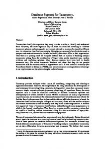
Probabilistic Database

!

Expand

Resulting Prob. Database

Collapse

!

Fig. 1.

Possible Worlds Semantics

In addition, even in situations where the base uncertain data is discrete, some queries (e.g. aggregates) can produce results that are very expensive to represent using discrete pdfs. The main reason is that the resulting uncertain attribute can have an exponential number of possible values. In such cases, one can save space as well as time by approximating with a continuous pdf. This is exactly what our model proposes. While our model is tailored towards representing continuous distributions, it is general enough to be used for modeling discrete uncertainty as well. In summary, the salient features of our model are: 1) It handle both continuous and discrete uncertainty (with arbitrary correlations) natively at the database level, and is consistent and closed under possible worlds semantics. 2) The first model for uncertain data that can accurately handle continuous pdfs. 3) The pdf approach leads to a more natural and efficient representation and implementation than a tuple uncertainty based approach. A. Possible Worlds Semantics The definition of relational operators for this model is based upon the Possible Worlds Semantics (PWS) [13] that has been commonly used for other work on uncertain databases. Under these semantics, a probabilistic relation is defined over a set of probabilistic events. Depending upon the outcome of each of these events, a possible world is defined. Thus given a probabilistic relation, we get a set of possible worlds corresponding to all possible combinations of the outcomes of the events in the relation. Figure 1 shows a graphical view of the possible worlds semantics. Given a probabilistic database and query θ to be evaluated over this database, conceptually we first expand the database to produce the set of all possible worlds. The query is then executed on each possible world. The resulting probabilistic database is defined as the database obtained by collapsing the possible worlds in which the query is satisfied. Consider a database table with uncertain attributes a and b, as shown in Table II. It consists of two probabilistic tuples. The first tuple represents a total of 4 possibilities: (i.e. {0, 1}, {0, 2}, {1, 1}, {1, 2}) and a single (certain) value for

TABLE II E XAMPLE OF P ROBABILISTIC TABLE a 0 1 7

Pr(a) 0.1 0.9 1.0

b 1 2 3

Pr(b) 0.6 0.4 1.0

TABLE III P OSSIBLE WORLDS Possible Worlds 0 7 0 7 1 7 1 7

Probability

1 3 2 3 1 3 2 3

0.06 0.04 0.54 0.36

the second tuple. The corresponding set of possible worlds are shown in Table III along with the associated probabilities for each world. The semantics of a query over this uncertain relation are defined as follows. The query is executed over each possible world (which has no uncertainty) to yield a set of possible results along with the probability of each result. The probability values of worlds that yield the same result are aggregated to yield the probability of that result for the overall query over the uncertain relation. Consider a selection query with predicate a < b, over the relation in Table II. Conceptually, this query is evaluated over each possible world. The probability that a tuple satisfies the query criterion is equal to the sum of the probabilities of the possible worlds in which the tuple satisfies the query. In practice, the number of possible worlds can be very large (even infinite for continuous uncertainty). The goal of a practical model is to avoid enumerating all possible worlds while ensuring that the results are consistent with PWS. Section III-C shows how our model handles this particular example. II. M ODEL In this section, we formally define our model for representing and querying a database with probabilistic data. We allow two kinds of attributes – uncertain (or pdf attributes) and certain (or precise) attributes. The model represents a set of database tables T, with a set of probabilistic schemas {(ΣT , ∆T ) : ∀T ∈ T} and a history Λ for each dependent set of attributes in T. A database table T is defined by a probabilistic schema (ΣT , ∆T ) consisting of a schema (ΣT ) and dependency information (∆T ). The schema ΣT is similar to the regular relational schema and specifies the names and data types of the table attributes (both certain and uncertain). The dependency information ∆T identifies the attributes in T that are jointly distributed (i.e., correlated). The uncertain attributes are represented by pdfs (or joint pdfs) in the table. In addition to pdfs, for each dependent group of uncertain attributes we store its history Λ. We will now describe each of these concepts in detail.

A. Uncertain Data types and Correlations There are two major kinds of uncertain data types that our model supports – discrete and continuous. These data types are represented using their pdfs. The uncertainty model in many real applications can be expressed using standard distributions. Our model has built in support for many commonly used continuous (e.g., Gaussian, Uniform, Poisson) and discrete (e.g., Binomial, Bernoulli) distributions. These distributions are stored symbolically in the database. The major advantage of using these standard distributions is efficient representation and processing. When the underlying data distribution cannot be represented using the standard distributions we revert to generic distributions – Histogram and Discrete sampling. The histogram distribution consists of buckets over the data domain, along with the probability density in each bucket. The discrete sampling simply consists of multiple valueprobability pairs. The bin size (or number of sampling points) is an important parameter that decides the trade-off between accuracy and efficiency. The simple pdf distributions discussed above can be used to represent 1-dimensional pdfs. But in many cases, there are intra-tuple correlations present within the attributes. For example, in a location tracking application, the uncertainty between the x- and y-coordinates of an object is correlated. These more complex distributions are supported in our model using joint probability distributions across attributes. For example, to represent the 2-D uncertainty in case of moving objects we represent the uncertainty by creating two uncertain attributes x and y which specify the x- and y-coordinates of the object, respectively. Instead of specifying two independent pdfs over x and y, we have a single joint pdf over these two attributes. The information about intra-tuple dependencies is captured by the schema dependency information ∆T . ∆T is a partition of all the uncertain attributes present in the table T . It consists of multiple sets of attributes that are correlated within a tuple. These sets are called dependency sets. It also contains singleton sets containing attributes that are uncertain but are not dependent on any other attributes. The attributes not listed in ∆T are assumed to be certain. To illustrate, let us consider a table T with schema ΣT = (a1 :d1 , a2 :d2 , a3 :d3 , a4 :d4 ), where di represents the data type of attribute ai . If all the attributes in the table are certain, ∆T = φ. On the other hand, if a1 , a2 and a3 are uncertain and a1 , a2 are correlated, this information is represented by defining the dependency information as ∆T = {a1 , a2 }, {a3 }. For the example presented in Table I, ΣT = {id : int, x : real} and ∆T = {x} (x represents the 1-D location). To model the location as a jointly distributed 2-D attribute, ΣT = {id : int, x : real, y : real} and ∆T = {x, y}. Consider the special case when all the attributes in a table T are jointly distributed (i.e. ∆T = {ΣT }). This extreme case captures tuple uncertainty as the complete value of the tuple is uncertain. The joint pdf over the attributes implicitly represents a group of dependent tuples. In addition, we can define tuples which are continuous and thus an infinite number

of alternatives are possible for each tuple. This representation is more powerful that the tuple uncertainty models in which each tuple can only have a finite number of alternatives. We allow the dependency information ∆T to contain phantom attributes which are not present in ΣT . These extra attributes and their corresponding joint distribution are needed for ensuring that the correlation information of the attributes that are projected out is not lost during projections (See Section III-B for more information). However, only the attributes in ΣT are visible to the user. Definition 1: A probabilistic tuple t of table T (ΣT , ∆T ) is represented by values t.aj for all certain attributes aj and pdf ft (Si ) for all sets of uncertain attributes t.Si ∈ ∆T . To be precise, let us define XSt i to be the random variable for an attribute set t.Si . Thus, ft (Si ) returns a pdf function that is defined over XSt i . That is, ft : Si → f (XSt i ). In the rest of this paper, whenever we refer to ft (Si ), it is understood that we are referring to the underlying distribution f (XSt i ). B. Partial pdfs In traditional databases, NULL is used to represent unknown or missing data. We also use NULL values in our model to signify missing attribute values. However, there is another way of representing missing data. The semantics of these two approaches differ from each other. To illustrate this point, let us consider the example presented in Table IV. The first tuple has missing (unknown) values for attribute b and c. However, the presence of the tuple itself is certain as the probability P r(b, c) adds up to 1. The other approach for representing missing data uses a closed world assumption to represent unknown information with partial pdfs. The ! probability that the second tuple exists in the table is 0.8 (= P r(b, c)) and thus with 0.2 probability the tuple does not exist in the table. Although both these approaches signify missing data their probabilistic interpretations are quite different. The usual definition of a pdf requires that it sums up (or integrates) to 1. We remove this restriction in our model in order to represent missing tuples with partial pdfs. The support for partial pdfs is crucial in our model to ensure that database operations such as selection are consistent with PWS. A partial pdf is a pdf where only the events associated with the existence of the tuple are explicitly represented. If the joint pdf of a tuple sums to x, then 1 − x is the probability that the tuple does not exist, under a closed world assumption. In this paper, we use the terms pdf and partial pdf interchangeably. TABLE IV E XAMPLE : M ISSING ATTRIBUTES VALUES VS M ISSING TUPLES a 1 2

b 2 NULL 4 4.1

c 3 NULL 7 3.7

Pr(b, c) 0.8 0.2 0.2 0.6

C. History As discussed in the previous section, we allow multiple attributes to be jointly distributed in our model. This flexibility makes the model very powerful in terms of data representation, by allowing intra-tuple dependencies (i.e. correlation between attributes). But for the model to be closed and correct under the usual database operations, we need to handle inter-tuple dependencies as well. History captures dependencies among attribute sets as a result of prior database operations. It is used to ensure that the results of subsequent database operations are consistent with PWS. This is described in more detail in Section III. A similar concept is used in many tuple uncertainty models to track correlations between tuples. [9] uses lineage and [14] uses factor tables to capture such dependencies. As we are interested in capturing historical dependencies between attributes of tuples, our concept of dependencies is different from this related work, which capture these dependencies on a per tuple basis. We maintain the history of uncertain attributes by storing the top-level ancestors of each dependency set in a tuple. The function Λ maps each pdf t.S of a tuple t, to a set of pdfs that are its ancestors. Definition 2: For a newly inserted tuple t in table T , from Λ(t.S) = t.S, ∀S ∈ ∆T . If a new pdf t" .S " is derived " pdfs t.Si via a database operation, then Λ(t" .S " ) = i Λ(t.Si ). In other words, the ancestors are the base pdfs which are inserted in the database by the user. We assume that the base tuples are independent. All the derived attributes point back to the base pdfs from which they are derived. Definition 3: If Λ(t.S1 ) ∩ Λ(t.S2 ) &= φ, then the nodes t.S1 and t.S2 are said to be historically dependent. Note that the deletion of a base tuple will cause dependency sets of its derived tuples to lose their ancestor information. Thus, while deleting a tuple from the base table, we first check if any other tuple in the database is referencing any dependency set within the tuple. If there is a reference, we delete the tuple but keep the dependency set and its pdf as a phantom node until its reference count falls to zero. Definition 2 assumes that the base tuples are historically independent. This is not limiting since a historical dependency between attribute sets of a base table, can be captured by creating a phantom ancestor and pointing the dependent attribute sets to this common phantom ancestor. III. P ROBABILISTIC O PERATIONS We begin by defining some basic operations on pdfs that underly the implementation of the usual database operations for our model. These operators are not directly accessible by users. One of the strengths of our model is that correctness with respect to PWS is achieved by manipulating the pdfs. Next, we present the usual relational operations under our model. The section concludes with a discussion of new operators that directly operate on the pdfs and are available to users as extensions to SQL.

A. Preliminaries

1 Similar implementation optimizations are possible for other operations presented in this paper. We skip their discussion in this paper due to space limitation.

(a)

(b)

0.03

0.25

0.025 0.2

pdf

pdf

0.02 0.015

0.15

0.1

0.01

0.05

0.005 0 -25

-20

-15

-10

-5

0

5

10

15

20

0 0

25

1

2

3

4

5

X

6

7

8

9

10

20

25

Y

(c) 0.009 0.008 0.007

Joint pdf

Here we describe some basic operations that are needed to define the usual relational database operations. marginalize(f, A): Given a pdf f over attributes Af , and a subset of attributes A ⊆ Af : the operation produces the pdf function f " over attributes A. This# is done by marginalizing the distribution f , i.e. f " = Af −A f . For discrete distributions, the integral is replaced by sum. It is easy to show the consistency wrt PWS because the probability of an event is the sum of probabilities of all the possible worlds in which the event occurs. floor(f, F ): Given a pdf f , on a domain D and given a subset F " ⊆ D, operation floor(f, F ) produces a new pdf f " such that values of f " (x) = 0 whenever x ∈ F and f " (x) = f (x) otherwise. This floor operation corresponds to a selection predicate. The values in F are those which do not pass the selection criteria and hence do not exist in the resulting pdf. Going by the PWS, this means that in the possible world where x takes the value in F , this tuple does not meet the selection criteria and hence it does not exist. Multiple floor operations can be successively applied over a pdf in any order and the result would be floor(f, F1 ∪...Fk ) regardless of the order in which they are applied. The application of floor on a symbolic distribution (e.g. Gaus) will, in general, result in a non-standard partial pdf. This partial pdf could be potentially captured by a histogram representation. But, we can optimize the floor operation (and subsequent operations) significantly, if we store symbolic floors to represent the flooring operation along with the original (symbolic) distribution. Our model has built-in support for simple symbolic floors which result from some common selection predicates. To illustrate, if the distribution of an attribute x is given by Gaus(5,1) and we apply the selection predicate x < 5, the resulting pdf will be floored when x ≥ 5 (and its value is given by Gaus(5,1) when x < 5). This resulting distribution is represented as [Gaus(5,1), Floor{[5, ∞]}] in our implementation.1 product(f1, f2 ): Given two pdfs f1 and f2 over attribute value sets S1 and S2 (in a given tuple t) respectively, the operation product gives their joint pdf f (over S " = S1 ∪ S2 ). We have to consider the following two cases: f1 and f2 are historically independent: In this case, f (x) = f1 (x1 )f2 (x2 ) where x ∈ S1 × S2 and x = (x1 , x2 ). To illustrate, assuming the pdfs shown in Figure 2(a), (b) are historically independent, the result of performing the product operation is shown in Figure 2(c). f1 and f2 are historically dependent: Let tj .Nj , 1 ≤ j ≤ m be the common ancestors of t.S1 and t.S2 (i.e. tj .Nj ∈ Λ(t.S1 ) ∩ Λ(t.S2 )). Each tj .Nj represents the distribution of an attribute set (Nj ) of a given tuple (tj ). Thus Nj denotes the set of attributes in tj .Nj . We define Cj = Nj ∩ S " and " Di = Si − Cj , i = 1 or 2. Thus Cj is the set of attributes

0.006 0.005 0.004 0.003 0.002 0.001 0

10

9

8

7

6

5

Y

Fig. 2.

4

3

2

1

-25 0

-20 -15

-10

-5

0

5

10

15

X

Example of product operation

that the ancestor tj .Nj shares with either S1 or S2 . D1 (D2 ) is the set of attributes in S1 (S2 ) that are not shared with any common ancestor. Let XSt be the random variable for an attribute set t.S. Let xtS be an instance of XSt . With these notations, the joint pdf of resulting set t.S " is: $ 0, if f (xtS1 ) or f (xtS2 ) = 0 t % f (xS ! ) = t m f (xtD1 )f (xtD2 ) j=1 f (xCjj ), otherwise

t t × XD × XCt11 × XCt11 . . . × XCtmm × XCtmm where, xtS ! ∈ XD 1 2 In other words, we first find the group of attribute sets (D1 , D2 and Cj , ∀j) that are independent of each other. We can multiply the distributions of these nodes as they are independent. But, that would ignore any floors that were applied during database operations from ancestor nodes tj .Nj to t.S1 or t.S2 . One potential solution is to keep track of all the operations and re-apply them2 but we observe that we can infer the final floors from the distributions of t.S1 and t.S2 . The regions where they were floored are the regions whose corresponding possible worlds did not “survive” the selection conditions. Thus, we propagate the floors of t.S1 and t.S2 to the joint distribution. This operator is used for defining selection and is further discussed in Section III-C. Note that this operator is associative and hence can be used over more than two pdfs as well.

B. Projections Given a table T , we define R = ΠA (T ) as the table which contains a tuple t" corresponding to each tuple t ∈ R (t → t" ), such that the resulting schema ΣR = A. The new dependency information ∆R can contain some of the attributes that are projected away. These attributes and their corresponding distributes are kept to ensure that we do not loose any floors associated with the projected out attributes. 2 This method, though correct, is very inefficient and will not scale with database size and number of operations.

# ∀Si ∈ ∆T , where Si ∩ A &= φ or ft (Si ) &= 1, we keep Si ∈ ∆R . A number of optimizations are possible to reduce the number of extra attributes that are kept in ∆R . For example, instead of the complete set Si , we can keep a subset Si" such that for each tuple, Si" functionally determine Si . The history of the new sets is updated to history of sets from which they are derived i.e. ∀t" ∈ R and ∀Sk ∈ ∆R where t → t" and Sk ⊆ Si (Si ∈ ∆T ), we have Λ(t" .Sk ) = Λ(t.Si ). Similar to other models for uncertain data, we do not address the issue of duplicate elimination in projections in this paper. This is because the concept of duplicate elimination for probabilistic data in general leads to complex historical dependencies. As part of our ongoing work, we are extending our model to address duplicate elimination. C. Selections Given a table T with attributes ΣT and a boolean predicate Θ(A) defined over a subset of attributes A of table T , the result of the selection operator is R = σΘ(A) (T ). If all the attributes in A are certain then we can simply use the “usual” definition of select operator to get the result. If not, selection will introduce new dependencies in the resulting set R, as explained below. Case 1 All the attributes ai ∈ A are certain: The schema ΣR = ΣT and the dependency information ∆R = ∆T . A tuple t ∈ T maps to a tuple t" ∈ R (i.e. t → t" ), if Θ(t.A) is true. That is, t" .ai = t.ai , ∀ certain ai and, ft! (Si ) = ft (Si ), ∀Si ∈ ∆R . The history is simply “copied over” for all the dependency sets i.e. ∀Si , Λ(t" .Si ) = Λ(t.Si ). As an example, the result of performing a selection σid=1 (T ) on the relation T presented in Table I would give us a single tuple t = [1, Gaus(20, 5)]. Case 2 At least one of the attributes ai ∈ A is uncertain: The schema ΣR = ΣT and dependency information ∆R = Ω(∆T ∪ {A}). The closure Ω is defined as follows: Definition 4: Given a set system {S1 , S2 , . . . , Sm } representing a hyper-graph, the closure Ω({S1 , S2 , . . . , Sm }) " produces a set system {S1" , S2" , . . . , Sm such that !} " " " S1 , S2 , . . . , Sm! represent the hyper-graph produced by merging all the connected components of {S1 , S2 , . . . , Sm }. To illustrate, if ∆T = {{a, b}, {c, d}, {e, f }} and A = {b, c, g} (g is certain), then Ω(∆T ∪ {A}) = {{a, b, c, d, g}, {e, f }}. Note that the sets {a, b} and {c, d} were merged due to the condition on A. The dependency set {e, f } was not affected as it is disjoint from A. Note that some of the certain attributes in T may become uncertain in R. Let us assume that a tuple t ∈ T maps to a tuple t" ∈ R (i.e. t → t" ). For all the certain attributes aj in R, we have t" .aj = t.aj (i.e., they are copied over). For the dependency sets that were disjoint from A, we do not need to do anything special. For the merged sets, we need to evaluate the resulting pdf. Thus, for ∀Sk ∈ ∆R , we have the following cases: Case 2(a) (A ∩ Sk = φ): This is the case when Sk does not share any attributes with the selection set A, and thus using Definition 4 and the fact that all Si ∈ ∆T are disjoint, we can

see that Sk is derived from exactly one attribute set Si ∈ ∆T , i.e. ft! (Sk ) = ft (Si ). Case 2(b) (A∩Sk &= φ): Using Definition 4 it is easy to see that (A ⊆ Sk ). In this case, Sk can be potentially derived from multiple attribute sets Si ∈ ∆T . These attribute sets Si are the sets for which (A ∩ Si &= φ). Let us assume fi , 1 ≤ i ≤ n are their respective pdfs. Sk consists of all the attributes in such sets Si and A. Let us assume that C is set of all certain attributes (C ⊂ A) and c is the value of C in t. We define the identify pdf f0 over C as f0 (c) = 1 and 0 otherwise. Now, we can derive the resulting pdf of Sk by performing a product operation over f0 , f1 , . . . , fm and flooring the resulting pdf in the region where Θ(A) is false. If the pdf of Sk is completely floored (i.e. the resulting probability of the tuple becomes 0), we remove that tuple from the result. Similar to the previous case, the histories of the new dependency sets are updated to the combined histories of sets from which they are derived i.e. ∀t" ∈ R and ∀Sk ∈ ∆R where t → t" , we have: & Λ(t" .Sk ) = Λ(t.Si ) ∀Si ⊆Sk ,Si ∈∆T

Consider the example shown in Table II. The probabilistic schema of that relation in our model would be represented as Σ = (a : int, b : int) and ∆ = {{a}, {b}}. There are two tuples t1 and t2 in that relation with pdfs ft1 ({a}) = Discrete(0 : 0.1, 1 : 0.9) and ft1 ({b}) = Discrete(1 : 0.6, 2 : 0.4) (this notation represents a discrete pdf, whose parameters xi : yi denote the probability yi for value xi ). Similarly, we can write the pdfs of t2 as ft2 ({a}) = Discrete(7 : 1.0) and ft2 ({b}) = Discrete(3 : 1.0). Applying a selection predicate σa4)

project(a)

Ta

T

a

b

ta1 Discrete(4:0.9, 2:0.1) ta2 Discrete(7:0.7)

Discrete(5:0.9)

Tb tb1

join

a b t'1 Discrete({4,5}:0.81, {2,5}:0.09) Discrete({7,5}:0.63) t'2 T1 (Incorrect!) Fig. 3.

a

b

Discrete({4,5}:0.9) Discrete({7,5}:0.63)

T2 (Correct)

Example illustrating histories

defined as follows. ΣR = ΣT1 ∪ ΣT2 and ∆R = ∆T1 ∪ ∆T2 . Let us assume a tuple t ∈ R is derived from tuples t1 ∈ T1 and t2 ∈ T2 (i.e. (t1 , t2 ) → t). ∀Sk ∈ ∆R and the corresponding Si ∈ ∆Tc , c = 1 or 2 we have, ft (Sk ) = ftc (Si ). Similarly, the history is also copied over for the new sets, Λ(t" .Sk ) = Λ(tc .Si ). Thus, conceptually joins are an application of cross-product followed by selection (as defined in Section III-C). The tuples that are produced as a result of join may contain some dependencies (implied by history Λ) which are not captured by the attribute dependencies (implied by ∆T ). We can, in principle, apply the algorithm explained in Section III-C to collapse the intra-tuple dependencies implied by Λ into ∆T . This decision will not affect the correctness or the semantics of the operations defined in this section but will have a significant effect on performance. The definition of the operations in this section assumes a lazy merging of dependencies and evaluation of joint pdfs. In practice, a combination of these techniques can be used to improve performance. Thus, the decision of whether to merge the intra-tuple dependencies eagerly or lazily is left to the implementation. Consider as an example, a table T with ΣT = (a : int, b : int) and ∆T = {{a, b}} as shown in Figure 3. We perform operations Πa (T ) and Πb (σb>4 (T )) to obtain the tables Ta and Tb (In this example, we do not need to keep the projected out attributes, as both the attributes a and b functionally determine each other in both the tuples). Clearly, ΣTa = (a : int) and ∆Ta = {{a}} for Ta ; and ΣTb = (b : int) and ∆Tb = {{b}} for Tb . Now, if we join Ta and Tb without considering historical dependencies we would get an incorrect result T1 . The tuple (2, 5) in t"1 can never exist because it do not exist in any possible world corresponding to table T . Similarly, the probability of tuple (4, 5) in T1 is incorrect as the pdfs of ta1 and tb1 share common ancestor t1 .{a, b} and thus the two events cannot be considered independent. Our model detects the historical dependency between tuples ta1

and tb1 and uses that information to correctly calculate the distribution of tuple t"1 in the final table T2 by considering the joint distribution of attributes a and b in T . In addition, as part of the tuple value (2, 3) (∈ T ) was floored in table Tb , we correctly floored that value in the distribution of t"1 .{a, b}. The correctness of the project and join operations with respect to the possible world semantics follows from the correctness of the selection operation and are thus omitted. Given the definition and the correctness of the selection, project, and join operations, we obtain the following theorem. Theorem 2: Our model is closed under selection, projection, and join operations. E. Operations on Probability Values We also allow queries based on the probability values of the tuples in our model. One example of such queries are threshold queries. Given a table T with probabilistic schema (ΣT , ∆T ), a threshold query R = σP r(A)>p (T ), where A ⊆ ΣT and p is the probability threshold, returns all tuples whose probability over the attribute set A is greater than p. As the operations on probability values act on the probabilistic model instead of a possible world, the possible worlds semantics described in Section I is not be used to define the semantics of these operations. In general, consider the boolean predicate given by Θ(S), where S = {P r(s1 ), P r(s1 ), . . . , P r(sm )} and si ⊆ ΣT . The result R of applying this selection on T consists of all tuples t ∈ T such that t satisfies Θ(S). The semantics of this operation and effect on histories is similar to Case 1 defined in Section III-C. IV. E XPERIMENTAL E VALUATION We have implemented our model in Orion, a publicly available extension to PostgreSQL that provides native support for uncertain data [8]. This system not only allows us to validate the accuracy of our methods in a realistic runtime environment, it also gives additional insight into the overall effect our techniques have on probabilistic query processing in an industrial-strength DBMS. The following experiments were conducted on a Sun-Blade-1000 workstation with 2 GB RAM, running SunOS 5.8, PostgreSQL 8.2.4, and Orion 0.2. Using a series of synthetically generated datasets, we explore the performance and accuracy of our model’s operations over pdfs. Each dataset consists of random “sensor readings,” using the schema Readings(rid, value). The uncertain pdfs (e.g. reported from the sensors) are Gaussians, with their means distributed uniformly from 0 to 100, and their standard deviations distributed normally using µ = 2 and σ = 0.5. We also generate numerous range queries, with midpoints distributed uniformly between 0 and 100, but with interval lengths distributed normally using µ = 10 and σ = 3. For simplicity, we omit the initial results of evaluating pdfs symbolically because they produce no approximation error and incur negligible overhead. Instead, our results focus on the relative performance of approximating symbolic pdfs with histograms as opposed to discrete sampling. Although it’s obvious

10

Average runtime (s)

15

Discrete Histogram

0

5

0.06 0.04 0.02 0.00

Average error

Discrete Histogram

5

10

15

20

25

0.5

1.0

Sample size Fig. 5.

B. Performance of Discretized PDFs For this experiment, we compare the performance of the aforementioned approximate representations. We fix the number of histogram bins at five and the number of discrete sample points at twenty-five, in order to compare runtimes at an equivalent level of accuracy. As shown in Figure 5, discretizing the data not only takes additional processing time,

3.0

Performance of Discretized PDFs

200

300

Join (with histories) Join (w/o histories) Project (with histories) Project (w/o histories)

0

Average runtime (s)

theoretically that histograms will generally outperform discrete representations, we wish to quantify the observed difference of these two approximations in our actual implementation. The first experiment shows the average error when answering range queries over histogram and discrete approximations of symbolic pdfs. We first discretize our dataset of random Gaussian pdfs, varying the number of sample points. Figure 4 shows the average approximation error of the cdf values returned at each sample size. The standard error over these averages is negligible. As expected, the histogram representation outperforms the discrete, even in the worst case (not shown). With only five sampling points, the accuracy is around ±0.01 probability mass. A discrete approximation requires over twenty-five sampling points, which greatly increases the size of each tuple and thus the overall I/O cost. Of course, a symbolic representation is both ideal in storage size and accuracy. We also show the standard deviation of the error values themselves, at each sample size, plotted only in the positive direction for clarity. As expected, a discrete representation has a considerably higher variance in approximation error than a histogram. Sometimes the error is quite large, for example in boundary cases when the query barely misses a discrete point. Continuous representations (including histograms) avoid this issue altogether because they can accurately estimate probability mass at arbitrary points. The difference in error is likely to be even greater in more complex pdfs.

2.5

Number of tuples (M)

Accuracy vs Sample Size

A. Accuracy vs Sample Size

2.0

100

Fig. 4.

1.5

1

2

3

4

5

Number of tuples (K) Fig. 6.

Overhead of Histories

but also incurs more disk reads, yielding a steeper rise in cost. Runtimes for the symbolic representation are just under the five-bin histogram times, but we do not show these here since they give an even higher level of accuracy. C. Overhead of Histories The final experiment shows the overall performance of the implementation of our proposed model inside PostgreSQL. We run two types of queries: joins over range queries (which involve floors and products), and projections of the resulting correlated data (triggering a collapse of the 2D pdfs). Figure 6 compares the average runtime of these queries with and without the overhead of maintaining histories for correctness. Note that ignoring histories will result in incorrect answers. The overhead shown in this figure ranges between 5-20%. Thus, although the proposed model is complex, it is efficient to implement and we pay a small overhead for correctness.

V. R ELATED W ORK

ACKNOWLEDGMENTS

Barbar´a et al. [12] and Dey et al. [15] proposed the first of the probabilistic models. Building on their work, many robust models for managing tuple uncertainty have been proposed recently. A significant challenge when modeling uncertain data is tracking arbitrary correlations both within and between tuples. These dependencies are not only present in real-world data, they are more commonly introduced by applying operations to independent base data. Benjelloun et al. have proposed a novel technique that combines uncertainty with data lineage to solve this problem [9]. The ProbView system [16] took a similar approach by propagating the formulas necessary to evaluating the resulting probabilities. Sen et al. have more recently proposed an alternative approach to represent tuple correlations using probabilistic graphical models [14]. They use factored representations of the relations to represent their dependencies. Antova et al. developed a compact representation called world-set decompositions which captures the correlations in the database by representing the finite sets of worlds [17]. Dalvi et al. introduced safe plans [18], [10] in an attempt to avoid probabilistic dependencies in queries. An important area of uncertain reasoning and modeling deals with fuzzy sets [1]. The work on fuzzy models is not immediately related to our work as we assume a probabilistic model. None of the aforementioned tuple uncertainty models can fully support continuous probability distributions. They suffer from loss of accuracy and efficiency. Parallel to this modeling effort, there has also been a lot of recent work on querying and indexing pdf attributes in databases [2], [3], [4], [5], [6], [7]. In previous work, we have proposed preliminary models for attribute uncertainty that overcome these limitations [19], [20]. We have also studied indexing methods for attribute uncertainty, both for continuous [6] and categorical [7] distributions. Apart from our work, there has been other work by [2], [3], [5] on indexing pdfs. However, none of this work considers PWS and hence its appeal is limited to solving specific problems. In this paper we have shown the first model for handling pdfs which can pave the way for more complex and useful operations involving pdfs.

This work was supported by NSF grants IIS 0534702, IIS 0415097, CCF 0621457, AFOSR award FA9550–06–1–0099, ARO grant DAAD19–03–1–0321 and by the Research Grants Council of Hong Kong CERG PolyU 5138/06E. We would also like to thank the Trio group at Stanford University for alerting us to an inconsistency in an earlier version of this model.

VI. C ONCLUSION We have presented a new model for handling arbitrary pdf (both discrete and continuous) attributes natively at the database level. Our approach allows a more natural and efficient representation and implementation for continuous domains. The model can handle arbitrary intra- and inter-tuple correlations. We show that our model is complete and closed under the fundamental relational operations of selection, projection, and join. In our previous work we have developed Orion – an extension of PostgreSQL that provides native support for attribute uncertainty with procedural semantics. We have extended Orion to support our new model. The experiments performed in Orion show the effectiveness and efficiency of our approach.

R EFERENCES [1] J. Galindo, A. Urrutia, and M. Piattini, Fuzzy Databases: Modeling, Design, and Implementation. Idea Group Publishing, 2006. [2] V. Ljosa and A. Singh, “APLA: Indexing arbitrary probability distributions,” in Proceedings of 23rd International Conference on Data Engineering (ICDE), 2007. [3] C. B¨ohm, A. Pryakhin, and M. Schubert, “The gauss-tree: Efficient object identification in databases of probabilistic feature vectors,” in Proceedings of International Conference on Data Engineering (ICDE), 2006. [4] R. Cheng, D. V. Kalashnikov, and S. Prabhakar, “Querying imprecise data in moving object databases,” IEEE Transactions on Knowledge and Data Engineering, vol. 16, no. 7, 2004. [5] A. Faradjian, J. Gehrke, and P. Bonnet, “GADT: A probability space ADT for representing and querying physical world,” in Proceedings of International Conference on Data Engineering (ICDE), 2002. [6] R. Cheng, Y. Xia, S. Prabhakar, R. Shah, and J. Vitter, “Efficient indexing methods for probabilistic threshold queries over uncertain data,” in Proceedings of International Conference on Very Large Data Bases (VLDB), 2004. [7] S. Singh, C. Mayfield, S. Prabhakar, R. Shah, and S. Hambrusch, “Indexing uncertain categorical data,” in Proceedings of 23rd International Conference on Data Engineering (ICDE), 2007. [8] “http://orion.cs.purdue.edu/,” 2006. [9] O. Benjelloun, A. D. Sarma, A. Halevy, and J. Widom, “ULDBs: Databases with Uncertainty and Lineage,” in Proceedings of the 32nd International Conference on Very Large Data Bases, 2006, pp. 953–964. [10] J. Boulos, N. Dalvi, B. Mandhani, S. Mathur, C. Re, and D. Suciu, “MYSTIQ: a system for finding more answers by using probabilities,” in Proceedings of ACM Special Interest Group on Management Of Data, 2005. [11] A. Deshpande and S. Madden, “MauveDB: supporting model-based user views in database systems,” in Proceedings of ACM Special Interest Group on Management Of Data, 2006, pp. 73–84. [12] D. Barbar´a, H. Garcia-Molina, and D. Porter, “The management of probabilistic data,” IEEE Transactions on Knowledge and Data Engineering, vol. 4, no. 5, pp. 487–502, 1992. [13] J. Y. Halpern, Reasoning about Uncertainty. The MIT Press, 2003. [14] P. Sen and A. Deshpande, “Representing and querying correlated tuples in probabilistic databases,” in Proceedings of 23rd International Conference on Data Engineering (ICDE), 2007. [15] D. Dey and S. Sarkar, “A probabilistic relational model and algebra,” ACM Transactions of Database Systems, vol. 21, no. 3, pp. 339–369, 1996. [16] L. Lakshmanan, N. Leone, R. Ross, and V. Subrahmanina, “Probview: A flexible probabilistic database system,” ACM Transactions on Database Systems, vol. 22, no. 3, pp. 419–469, 1997. [17] L. Antova, C. Koch, and D. Olteanu, “10ˆ10ˆ6 worlds and beyond: Efficient representation and processing of incomplete information,” in Proceedings of 23rd International Conference on Data Engineering (ICDE), 2007. [18] N. Dalvi and D. Suciu, “Efficient query evaluation on probabilistic databases,” in Proceedings of International Conference on Very Large Data Bases (VLDB), 2004. [19] R. Cheng, S. Singh, and Prabhakar, “U-DBMS: A database system for managing constantly-evolving data,” in Proceedings of Very Large Databases Conference (VLDB), 2005. [20] R. Cheng, S. Singh, S. Prabhakar, R. Shah, J. Vitter, and Y. Xia, “Efficient join processing over uncertain data,” in Proceedings of ACM 15th Conference on Information and Knowledge Management (CIKM), 2006.