1: The itinerary and track circuit level view of a station. Train .... S+ to indicate that a train is reaching an entry point of a ring section S, (corre- spondingly ...
This is a post-peer-review, pre-copyedit version of an article published in FMICS 2014 The final authenticated version is available online at: https://doi.org/10.1007/978-3-319-10702-8_8
Deadlock Avoidance in Train Scheduling: a Model Checking Approach ? Franco Mazzanti, Giorgio O. Spagnolo, Simone Della Longa, and Alessio Ferrari Istituto di Scienza e Tecnologie dell’Informazione “A.Faedo”, Consiglio Nazionale delle Ricerche, ISTI-CNR, Pisa, Italy
Abstract. In this paper we present the deadlock avoidance approach used in the design of the scheduling kernel of an Automatic Train Supervision (ATS) system. The ATS that we have designed prevents the occurrence of deadlocks by performing a set of runtime checks just before allowing a train to move further. For each train, the set of checks to be performed at each step of progress is retrieved from statically generated ATS configuration data. For the verification of the correctness of the logic used by the ATS and the validation of the constraints verified by the runtime checks, we define a formal model that represents the ATS behavior, the railway layout, and the planned service structure. We use this formal model to verify both the absence of deadlocks and absence of false positives (i.e., cases in which a train is unnecessarily disallowed to proceed). The verification is carried out by exploiting the UMC model checking verification framework locally developed at ISTI-CNR.
1
Introduction
One of the pillars of current industry-related research in Europe is the development of intelligent green transport systems managed by smart computer platforms that can automatically move people within the cities, while at the same time ensuring safety of passengers and personnel. In particular, in the metro signaling domain, the increasing demand for automation have seen the raise of Communications-based Train Control (CBTC) systems as a de-facto standard for coordinating and protecting the movements of trains within the tracks of a station, and between di↵erent stations. In CBTC platforms, a prominent role is played by the Automatic Train Supervision (ATS) system, which automatically dispatches and routes trains within the metro network. In absence of delays, the ATS coordinates the movements of the trains by adhering to the planned timetable. In presence of delays, the ATS has to provide proper scheduling choices to guarantee a continuous service and ensure that each train reaches its destination. In particular, this implies that the ATS shall necessarily avoid the occurrence of deadlock situations, i.e., situations where a group of trains block each other, preventing in this way the completion of their missions. ?
This work was partially supported by the PAR FAS 2007-2013 (TRACE-IT) project and by the PRIN 2010-2011 (CINA) project.
This paper presents the experience of ISTI-CNR in the design of the scheduling kernel of an ATS system. The component was designed within the framework of an Italian project, namely “Train Control Enhancement via Information Technology” (TRACE-IT) [1]. The project concerns the specification and development of a CBTC platform, and sees the participation of both academic and industrial partners. Within the project, a prototype of the ATS system has been implemented, which operates on a simple but not trivial metro layout with realistic train missions. To address the problem of deadlock avoidance in our ATS prototype, we have decided to develop sound solutions based on formal methods. In a short preliminary work [2], we have outlined a model-checking approach for the problem of deadlock avoidance. Such an approach included several manual steps, and did not consider the presence of false positives (i.e., cases in which a train is unnecessarily disallowed to proceed). The approach presented in this paper the principles of the previous work to define a more structured, semiautomated approach that can deal with realistic circular missions. Furthermore, the current strategy exploits the usage of model checking also to address the problem of false positives. The ATS that we have designed prevents the occurrence of deadlocks by performing a set of runtime checks just before allowing a train to move further. The set of checks to be performed is retrieved from statically generated configuration data that are validated by means of model checking. Our approach to produce valid configuration data starts with the automatic identification of a set of basic cases of deadlocks. This goal is achieved by statically analysing the missions of all the trains, and providing a set of preliminary constraints that can be used to address the basic cases of deadlocks. Then, we build a formal model of the scheduling kernel of the ATS that includes the constraints associated to the basic cases of deadlock. We use such a formal model to verify the absence of complex cases of deadlocks, and to assess the absence of false positive cases. To this end, we apply model checking by means of the UMC (UML Model Checker) tool, which is a verification environment working on UML-like state machines [3]. When complex cases of deadlock are found, the formal model is updated with additional checks to address such cases. The validation process iterates until the ATS configuration data are proven to avoid all possible cases of deadlocks. The verification of the configuration data for the full railway yard is performed by decomposing it into multiple regions to be analysed separately, and by proving that the adopted decomposition allows extending the results to the full layout. The paper is structured as follows. In Sect. 2, we illustrate an abstract model of the ATS, together with the metro layout and the missions of our ATS prototype. In Sect. 3, the basic cases of deadlocks are described, and the approach to identify and automatically avoid such cases is outlined. Sect. 4 explains how complex cases of deadlocks can occur, and introduces the problem of false positives. Sect. 5 describes the formal model provided for the ATS and the approach adopted to verify the absence of deadlocks and false positives. In Sect. 6, we describe how we have partitioned the full layout. Sect. 7 reports the most relevant works related to ours, and Sect. 8 draws conclusions and final remarks.
2
An Abstract Model of the System
The abstract behavior of the kernel of the ATS system can be seen as a state machine. This state machine has a local status recording the current progress of the train missions and makes the possible scheduling choices among the trains which are allowed to proceed. BCA01
Piazza Università
Piazza Università I BCA02
3
4
6
14020
14021
14022
I
14301
14012
14011
14010
BCA501
BCA502
II 5
II
(a) Itinerary level view
14302
(b) Track circuit level view
Fig. 1: The itinerary and track circuit level view of a station Train movements can be observed and modeled at di↵erent levels of abstractions. In Figure 1 we show two levels of abstraction of the train movement, namely the itinerary level view and the track circuit level view. An itinerary is constituted by the sequence of track circuits (i.e., independent line segments) that must be traversed for arriving to a station platform from an external entry point, or for leaving from a station platform towards an external exit point. Track circuits are not visible at the itinerary level view, which is our level of observation of the system for the deadlock-avoidance problem. Instead, at the interlocking management level, we would be interested in the more detailed track circuit level view, because we have to deal with the setting of signals and commutation of switches for the preparation of the requested itineraries. Notice that it is task of the interlocking system (IXL) to ensure the safety of the system by preparing and allocating a requested itinerary to a specific train. At the ATS level it is just a performance issue the need to avoid the issuing of requests which would be denied be the IXL, or to avoid sequences of safe (in the sense risk free) train movements but which would disrupt the overall service because of deadlocks. Parco della Vittoria
III Via Accademia I
green
11 II
22
Piazza Università BCA01
33 red
BCA02
I
6
44
Via Verdi I
77
BCA03
Piazza Dante I
9 9
10 10
II
II
II
55
88
11 11
Vicolo Corto Vicolo Stretto I I yellow
Viale Monterosa I
31 31
30 30
28 28
II
BCA04
II
32 32
blu
e
III 12 12
Via Roma Via Marco Polo
15 15
gree
II 13 13
16 16
20 20
17 17
Viale dei Giardini
red >>
yell
I 18 18
22 22
I 23 23
n >>
ow
blu
>>
II 24 24
III 25 25
e>
> IV
26 26
27 27
BCA05
29 29
Fig. 2: The yard layout and the missions for the trains of the green, red, yellow and blue lines In our case, the overall map of the railway yard which describes the various interconnected station platforms and station exit/entry points (itinerary endpoints) is shown in Figure 2. Given our map, the mission of a train can be seen as a sequence of itinerary endpoints. In particular, the service is constituted by eight trains which cyclically start their missions at the extreme points
of the layout, traverse the whole layout in one direction and then return to their original departure point. The missions of the eight trains providing the green/red/yellow/blue line services shown in Figure 2, are represented by the data in Table 1. Green1: [1,3,4,6,7,9,10,13,15,20,23,22,17,18,11,9,8,6,5,3,1] Green2: [23,22,17,18,11,9,8,6,5,3,1,3,4,6,7,9,10,13,15,20,23] Red1: [2,3,4,6,7,8,9,10,13,15,20,24,22,17,18,11,9,8,6,5,3,2] Red2: [24,22,17,18,11,9,8,6,5,3,2,3,4,6,7,8,9,10,13,15,20,24] Yellow1:[31,30,28,27,11,13,16,20,25,22,18,12,27,29,30,31] Yellow2:[25,22,18,12,27,29,30,31,30,28,27,11,13,16,20,25] Blue1: [32,30,28,27,11,13,16,20,26,22,18,12,27,29,30,32] Blue2: [26,22,18,12,27,29,30,32,30,28,27,11,13,16,20,26]
Table 1: The data for the missions In absence of deadlock avoidance checks, in our abstract model, trains are allowed to move from one point to the next under the unique condition that the destination point is not assigned to another train. This transition is modeled as an atomic transition, and only one train can move at each step. We are interested in evaluating the traffic under any possible condition of train delays. Therefore we abstract completely away from any notion of time and from the details of the time schedules. Indeed, if we consider all the possible train delays, the actually planned times of the time table become not relevant.
3
The basic cases of deadlock
A basic deadlock occurs when we have a set of trains (each one occupying a point of the layout) waiting to move to a next point that is already occupied by another train of the set. In our railway scenario this means that we have a basic deadlock when two trains are trying to take the same itinerary in opposite directions, or when a set of trains are moving around a ring which is completely saturated by the trains themselves. We consider as another case of basic deadlock the situation in which two trains are trying to take the same linear sequence of itineraries in opposite directions. 1
2
A B
3
4
C
5
6
7
D
9
8
Fig. 3: A a sample selection of four basic critical sections from the full layout For example, if we look at the top-left side of our yard layout we can easily recognize four of these zones in which the four Green and Red trains might create one of these basic deadlocks (see also Figure 3): a) The zone A [1-3] when occupied by Green1 and Green2. b) The zone B [2-3] when occupied by Red1 and Red2. c) The zone C [3-4-6-5] when occupied by the four Green and Red trains.
d) The zone D [6-7-9-8] when occupied by the four Green and Red trains.
The first step of our approach to the deadlock free scheduling of trains consists in statically identifying all those zones of the railway layout in which a basic deadlock might occur. We call these zones basic critical sections. We have already seen the two basic kinds of critical sections, namely ring sections and linear sections, which are associated to the basic forms of deadlocks mentioned before. Given a set of running trains and their missions, the set of basic sections of a layout are statically and automatically discovered by comparing the various missions of all trains. In particular, linear sections are found by comparing all possible pairs of train missions. For example if we have that: Train1: [ ..., a, x, y, z, b, ...] Train2: [ ..., c, z, y, x, d, ...]
a
b x
y
z c
d
then (x,y,z) constitutes a basic linear section of the layout. Similarly if we have for example three trains such that: Train1: [ ..., x, y, ...] Train2: [ ..., y, z, ...] Train3: [ ..., z, x, ...]
x
z
y
then (x,y,z) constitutes a basic ring section of the layout. The next step of our approach consists in associating one or more counters to the critical sections in order to monitor at execution time that the access to them will not result in a deadlock. It is indeed evident that if we allow at most N-1 trains to occupy a ring section of size N no deadlock can occur on that ring. Similarly, in the case of linear sections, we could use two counters (each one counting the trains moving in one direction) and make sure that one train enters the section only if there are no trains coming from the opposite side (while still allowing several trains to enter the section from the same side). When a train is allowed to enter a basic critical section the appropriate counter is increased; when the train is no longer a risk for deadlocks (e.g. moves to an exit point of the section) the counter is decreased. The above policy can be directly encoded in the description of the train missions by associating to each itinerary endpoint the information on which operations on the counters associated to the entered/exited sections should be performed when moving to that endpoint. We call the description of the train missions extended with this kind of information extended train mission. Let S be a generic name of a section. In the following we will use the notation S+ to indicate that a train is reaching an entry point of a ring section S, (correspondingly increasing its counter), and the notation S- to indicate that a train is reaching an exit point of section S (correspondingly decreasing its counter). The notation SR+ (SR-) indicates that a train is reaching the entry (exit) point of a linear section S from when arriving from its right side. The notation SL+ (SL-) indicates that a train is reaching the entry (exit) point of a linear section S from when arriving from its left side.
The cases of deadlocks over the basic sections shown in Figure 3 can be avoided by extending the missions of the trains of the green and red lines (originally shown in Table 1) in the following way: Sections: [A, B, C max 3, D max 3] Train Missions: Green1: [(AL+)1,(AL-,C+)3,4,(C-,D+)6,7,(D-)9,10,13,15,20,23, 22,17,18,11,(D+)9, 8,(D-,C+)6,5,(C-,AR+)3,(AR-)1 ] Green2: [23,22,17,18,11,(D+)9,8,(D-,C+)6,5,(C-,AL+,AR+)3,(AR-)1, (AL-,C+)3,4,(C-,D+)6,7,(D-)9,10,13,15,20,23 ] Red1: [(BL+)2,(BL-,C+)3,4,(C-,D+)6,7,(D-)9,10,13,15,20,24, 17,18,11,(D+)9,8,(D-,C+)6,5,(C-,BR+)3,2 ] Red2: [24,22,17,18,11,(D+)9,8,(D-,C+)6,5,(C-,BL+,BR+)3,(BR-)2, (BL-,C+)3,4,(C-,D+)6,7,(D-)9,10,13,15,20,24 ]
Given the discovered set of basic sections, the description of the extended train missions for all running trains can be automatically computed without e↵ort. By performing such an initial static analysis on the overall service provided by our eight train missions shown in Figure 2 we can find eleven basic critical sections (see Figure 4) and automatically generate the corresponding extended mission descriptions for all trains. All this automatically generated data about critical sections and extended missions will be further analyzed and validated before being finally encoded as ATS configuration data and used by the ATS to perform at runtime the correct train scheduling choices. 23
16
20
17
22
27
28
30 13
29 11
18
7
6
15
9
8 13
20 3
11
18
17
4
6
22 5
15
13
11
18
26
20
17
22
25
16
20
24
1
3
31
3 13
2 11
18
17
30
30
32
22
Fig. 4: All the basic critical sections of the overall layout
4
From basic to composite sections
Our set of basic critical sections actually becomes a new kind of resource shared among the trains. When moving from one section to another, a train may have to release one section and acquire the next one. Again, this behavior can be subject to deadlock. Let’s consider the example of regions A, B, C shown in Figure 5.
A B
3
1 2
4
6
5
C
A
3
1 2
B
4
6
5
C
Fig. 5: Deadlock situations over the composition of basic critical sections In the left case (the right case is just an analogous example), train Green2 cannot exit from critical section C because it is not allowed to enter critical section A. Moreover, train Green1 is not allowed to leave critical section A because it is not allowed to enter critical section C. The deadlock situation that is generated in the above case is not a new case of deadlock introduced by our deadlock avoidance mechanism, but just an anticipation of an unavoidable future deadlock (of the basic kind) which would occur if we allow one of the two trains to proceed. To solve these situations, we can introduce two additional composite critical section E and F respectively over the points [1-3-4-6-5], (section A plus section C) and [2-3-4-6-5] (section B plus section C), which are allowed to contain at most three of the trains Green1, Green2, Red1, Red2). These new sections are shown in Figure 6a. The missions of the Green and Red trains are correspondingly updated to take into consideration also these new sections. E
E A B
1 2
3
6
4
A
C
5
B
Green
3
1 2
Re
d
Re
d
5
F
(a) The composite sections E and F
6
4 en Gre C
F
(b) A potential deadlock caused by false positives
Fig. 6: Composite sections and new deadlock case It is very important that our mechanism does not give raise to false positive situations, i.e, situations in which a train is unnecessarily disallowed to proceed. False positive situations, in fact, not only decrease the efficiency of the scheduling but also risk to propagate to wider composite sections, creating even further cases of false positives or deadlocks. Let us consider the situation shown in Figure 6b. The red train in 2 is not allowed to proceed in point 3 because section E already contains its maximum of three trains. The same occurs for the green train in point 1 (section F already has three trains). As a consequence nobody can progress, while, on the contrary, nothing bad would occur if the red train in 2 was allowed to proceed. As we build greater composite sections it becomes extremely difficult to manually analyze the possible e↵ects of the choices. We need a mechanical help for exhaustively evaluating the consequences of our choices, discover possible new cases of deadlock involving contiguous or overlapping critical sections, and completely eliminate potential false positives situations from the newly introduced composite critical sections. As shown in Figure 7, we will rely on model checking approach for starting a sequence of iterations in which new problems in terms
Train Missions
Validated ATS Data
Initial model (handling basic deadlocks)
No more deadlocks or false positives
Model Checking
New deadlocks or false positives New sections, counters, and updated missions
Fig. 7: The ATS configuration data validation process
of deadlocks are found are resolved by creating and managing new sections in an incremental way.
5
A verifiable formal model of the system
The behavior of the abstract state machine describing the system can be rather easily formalized and verified in many ways and using di↵erent tools. We have chosen to follow a UML-like style of specification and exploit our in-house UMC framework. UMC is an abstract, on-the-fly, state-event based, verification environment working on UML-like state machines [3]. Its development started at ISTI in 2003 and has been since then used in several research projects. So far UMC is not really an industrial scale project but more an (open source) experimental research framework. It is actively maintained and is publicly usable through its web interface (https://fmt.isti.cnr.it/umc). In UMC a system is described as a set of communicating UML-like state machines. In our particular case the system is constituted by a unique state machine. The structure of a state machine in UMC is defined by a Class declaration which in general has the following structure: class is Signals: Operations: Vars: Behavior: end
The Behavior part of a class definition describes the possible evolutions of the system. This part contains a list of transition rules which have the generic form:
--> {[ ] / }
Each rule intuitively states that when the system is in the state SourceState, the specified EventTrigger is available, and all the Guards are satisfied, then all the Actions of the transition are executed and the system state passes from SourceState to TargetState (we refer to the UML2.0 [4] definition for a more rigorous definition of the run-to-completion step). In UMC the actual structure of the system is defined by a set of active object instantiations. A full UMC model is defined by a sequence of Class and Objects declarations and by a final definition of a set of Abstraction rules. The overall behavior of a system is in fact formalized as an abstract doubly labelled transition system (L2TS), and the Abstraction rules allow to define what we want see as labels of the states and edges of the L2TS. The temporal logic supported by UMC (which has the power of full µ-calculus but also supports the more high level operators of CTL/ACTL uses this abstract L2TS as semantic model and allows to specify abstract properties in a way that is rather independent from the internal implementation details of the system [5]. It is outside the purpose of the paper to give a comprehensive description of the UMC framework (we refer to the online documentation for more details). We believe instead that a detailed description of fragment of the overall system can give a rather precise idea of how the system is specified. To this purpose, we take into consideration just the top leftmost region of the railway yard as show by Figure 8, which is traversed only by the four trains of the green and red lines. Via Accademia I BCA01 1
3
Piazza Università I BCA02 6 4
Via Verdi I 7
II
II
II
2
5
8
91 BCA03 9
92 93 94
Fig. 8: The top-left region of the full railway yard Our UMC model is composed of a single class REGION1 and a single object SYS. class REGION1 is ... end REGION1 SYS: REGION1 -- a single active object Abstractions { }
In our case the class REGION1 does not handle any external event, therefore the Signals and Operations parts are absent. The Vars part, in our case contains, for each train, the vector describing its mission, and a counter recording the current progress of the train (an index of the previous vector). E.g. G1M: int[]:= [1,3,4,6,7,9,92,91,9,8,6,5,3,1]; --mission of train Green1 G1P: int := 0; --progress inside mission of train Green1, i.e. index inside G1M
Similar mission and progress data is defined for the other trains as G2M, G2P (train Green2), R1M, R1P (train Red1), R2M, R2P (train Red2). As we have seen in the previous sections, in this area we have to handle six critical sections, called A, B, C, D, E, F. For the sake of simplicity, in in this case we handle the linear A and B critical sections as if they were rings of size 2 (which allow at most one train inside them). We use six variables to record the limits of each section, and other six variables to record the current status of the various sections, properly initialized with the number of the trains initially inside them. MAXSA: int :=1; -- section MAXSB: int :=1; -- section MAXSC: int :=3; -- section MAXSD: int :=3; -- section MAXSE: int :=3; -- section MAXSF: int :=3; -- section SA: int :=1; SB: int :=1; SD: int :=0; SE: int :=1;
A: [1,3] (see Figures 3, 6a and 8) B: [2,3] C: [3,4,5,6] D: [6,7,9,8] E: [1,3,4,5,6] F: [2,3,4,5,6] SC: int :=0; SF: int :=1;
For each train, the set of section updates to be performed at each step is recorded into another table which has the same size of the train mission. We show below the table G1C which describes the section operations to be performed by train Green1 during its progress: G1C: int[] := -- Section counters updates to be performed by train Green1 --A,B,C,D,E,F [[1,0,0,0,1,0], --1 [0,0,0,0,0,0], --92-91 [-1,0,1,0,0,1], --1-3 [0,0,0,1,0,0], --11-9 [0,0,0,0,0,0], --3-4 [0,0,0,0,0,0], --9-8 [0,0,-1,1,-1,-1], --4-6 [0,0,1,-1,1,1], --8-6 [0,0,0,0,0,0], --6-7 [0,0,0,0,0,-1], --6-5 [0,0,0,-1,0,0], --7-9 [1,0,-1,0,0,0], --5-3 [0,0,0,0,0,0], --9-92 [0,0,0,0,0,0]]; --3-1
The element i of the table records the increments or decrements that the train must apply to the various section counters to proceed from step i to step i+1 of its mission. For example, in order to proceed, at step 1, from endpoint 1 to endpoint 3, train Green1 must apply the updates described in the element [-1,0,1,0,0,1], i.e., decrement the counter of section A, and increment the counters for sections C and F. In the Behavior part of our class definition we will have one transition rule for each train, which describes the conditions and the e↵ects of the advancement of the train. In our case there is no external event which triggers the system transitions, therefore they will be controlled only by their guards. In the case of train Green1, for example, we will have the rule: 01: 02: 03: 04: 05: 06: 07: 08: 09: 10: 11:
s1 -> s1 { - [(G1P
MAXSA MAXSB MAXSC MAXSD MAXSE MAXSF
-> -> -> -> -> ->
DEAD DEAD DEAD DEAD DEAD DEAD
In this way we can check the absence of false positives by verifying the formula: not EF (DEAD and EF ARRIVED)
Which states that does not exists a path (E) which eventually reches (F) a state that labelled DEAD, and from which exists (E) a continuation of the path which eventually reaches (F) a state in which all trains are in their destination. Unfortunately the above formula false, and that allows discovering several other cases of false positives, (like the one shown in Figure 9) whose removal requires a more refined use of the counters (the final version of the code can be found at http://fmt.isti.cnr.it/umc/examples/traceit/). If we want to check again the absence of deadlocks in this second kind of model we can now modelcheck the formula: A[(EF ARRIVED) U (DEAD or ARRIVED)]
This is a typical branching time formula, which states two things. The first is that all paths will eventually reach a state labelled as DEAD or ARRIVED. The second is that for all intermediate states of these paths there is scheduling choice that allows driving all trains to destination (EF ARRIVED) . In this case the size of the generated statespace is 10493 configurations and the evaluation time is less than two seconds. E A B
1
Green
3
2
Red
Red
6
4 5
een
Gr
C
F
Fig. 9: Another case of false positive for section E
6
Partitioning the Full Model
Sometimes the scheduling problem might be too complex to be handled by the model checker. In these cases, it is useful to split the overall layout into subregions to be analyzed separately. In particular, in the system used as our case study, we have four trains moving along the red-line and green-line service, and four other trains moving along the yellow-line and blue-line service. In we consider all the possible interleavings of eight trains each one performing about 20 steps, we get a system with about 208 configurations. Most model checkers (and UMC among them) may have difficulties in performing an exhaustive analysis over a system of this size, therefore it is useful to consider a possible splitting of the
overall layout. In our case we have considered a partitioning of the system as shown in Figure 10. The analysis of region 1 has been performed following the approach outlined in the previous sections, and has led to the management of six critical sections. Via Accademia BCA01 I 1
3
Piazza Università BCA02 I 6 4
Via Verdi I 7
II
II
II
2
5
8
BCA03 9 Parco della Vittoria I
III BCA03
Piazza Dante I
9
10
Via Roma Via Marco Polo
II
II 13
20
16
I
II 18
11
25
IV
Viale dei Giardini
12
24
III 22
17
III
BCA05
23
15
26
27
Vicolo Corto I
Vicolo Stretto I
31
30
28
II
BCA04
II
Viale Monterosa BCA05 I
32
27
29
Fig. 10: The three regions partitioning the full layout The analysis of region 3 is similar to the previous one, and leads to the introduction of further four critical sections. The analysis of region 2 is more complex, being bigger and with 8 trains inside it. The analysis does not reveals any new cases of deadlocks or false positives, therefore the critical section remain the basic sections already discovered with our static analysis (shown in Figure 11). The statespace size of the model for region 2 is 6,820,504 configurations and its verification takes a few minutes. In general, it is not true that the separate analysis of the single regions in which a layout is partitioned actually reveals all the possible deadlocks of the full system. For this being true it is necessary that the adopted partitioning does not cut (hiding it from the analysis) any critical section that overlaps two regions. Since we know from our static analysis were are positioned the basic critical sections for the layout, and we know that composite sections can only extend over contiguous/overapping basic sections, it is sufficient to partition the system in such a way that each region encloses completely a closed group of connected basic sections. Parco della Vittoria I
III BCA03 9
Piazza Dante I 10
Via Roma Via Marco Polo
11
III 12
II
II 13
16
20
I
II
BCA05
23
15
18
17
24
III 22
Viale dei Giardini
27
Fig. 11: Four critical sections in region 2
25
IV 26
7
Related Work
The problem of deadlock avoidance in train scheduling has been studied since the 80s. In one of the first works on the subject, Petersen and Taylor [6] propose a solution based on dividing the line into track segments and using algebraic relationships to represent the model logic. The Petersen and Taylor algorithm is able to determine a deadlock in a simple network but is not able to deal with complex networks, which include fleets moving in more than two directions [7]. Mills and Pudney [8] propose a labeling algorithm similar to the Petersen and Taylor algorithm, presenting high computational efficiency but only suitable for simple networks with only single lines and crossing loops. In [9] and [10], Pachl describes two solutions to the deadlock problem. One is the Movement Consequence Analysis (MCA), derived from studies on routing techniques for stochastic networks. This solution, however, is based on the analysis of the next N movements of the train, without specifying how to determine the correct value of N. The second solution, Dynamic Route Reservation (DRR), is an evolution of MCA and is based on authorizing the movement of a train only after the reservation of a portion of the route. This approach does not guarantee the absence of deadlock and can lead to false positives. In [7], Cui describes an application of the Bankers Algorithm to the deadlock problem. Movement tasks are modeled as processes and track segments as resources. Requests are approved if all the processes can obtain all the required resources. The algorithm can lead to false positives and it is time-consuming. The author proposes various improvements to reduce false positives and improve general performance. Mittermayr [11] uses Kronecker Algebra to model the train routes and build an evolution graph, subsequently reduced to the relevant synchronizing nodes. This approach has been used to model additional constraints such as alternative routes, long trains that occupy more than one track circuit, synchronization in case of route overtaking and connection. The solution avoids false positives and false negatives. This approach, however, requires the Scheduler to have access to the evolution graph in order to successfully schedule trains dynamically.
8
Conclusions
The development of solutions to the problem of deadlock avoidance in train scheduling is a complex and still open task [12]. Many studies have been carried out on the subject since the early ’80s, but most of them are related to normal railway traffic, and not to the special case of driverless metropolitan systems. Automatic metro systems indeed may express some original properties, e.g., the difficulty of changing the station platform on which a train should stop, or the fact that all trains keep moving continuously, which makes the problem rather di↵erent from the classical railway case. The project under which this study has been carried out is still in progress, and the actual ATS prototype in under development. There are many directions in which this work is going to proceed. For example, we want to see if the model checking / model refinement cycles for
the detection and management of critical sections could be in some way fully automatized removing the human intervention for the generation of the final validated ATS configuration data. A further interesting evolution would be the generation and validation of the critical sections data directly from the inside of the ATS. This would allow to automatically handle at run time also the dynamic change of the itinerary of the trains. The current metro-line oriented approach could be further generalized to a wider railway oriented setting by taking into consideration the train and platform lengths, or the possibility of specifying connections and overtakings among trains. At a first look the handling of these aspects should require only minor updates of our current approach.
References 1. Ferrari, A., Spagnolo, G.O., Martelli, G., Menabeni, S.: From commercial documents to system requirements: an approach for the engineering of novel CBTC solutions. Int. Journal on STTT (2014) 1–21 2. Mazzanti, F., Spagnolo, G.O., Ferrari, A.: Design of a deadlock-free train scheduler: a model checking approach. In: to appear in Proc. of NFM’14. (2014) 3. Gnesi, S., Mazzanti, F.: An abstract, on the fly framework for the verification of service-oriented systems. In: Rigorous Software Engineering for Service-Oriented Systems. Volume 6582 of LNCS., Springer (2011) 390–407 4. OMG: Object Management Group, UML Superstructure Specification http://www.omg.org/spec/UML/2.4.1 (2006) 5. ter Beek, M.H.and Mazzanti, F., Gnesi, S.: CMC-UMC: A Framework for the Verification of abstract Service-Oriented Properties. In: Proceedings of the 2009 ACM symposium on Applied Computing, ACM (2009) 2111–2117 6. Petersen, E., Taylor, A.: Line Block Prevention in Rail Line Dispatch and Simulation Models. INFOR Journal (21) (1983) 46–51 7. Cui, Y.: Simulation-based hybrid model for a partially-automatic dispatching of railway operation. In: Ph.D. Thesis Universitat Stuttgart. (2009) 8. Mills, R., Pudney, P.: The e↵ects of deadlock avoidance on rail network capacity and performance. In: MISG: Mathematics in Industry Study Group, Hewitt, J. (2003) 9. Pachl, J.: Avoiding deadlocks in synchronous railway simulations. In: International Seminar on Railway Operations Modelling and Analysis. (2007) 359–369 10. Pachl, J.: Deadlock avoidance in railroad operations simulations. In: PROMET Traffic&Transportation. Number 11-0175 (2012) 359–369 11. Mittermayr, R., Blieberger, J., Sch¨ obel, A.: Kronecker Algebra based Deadlock Analysis for Railway Systems. PROMET - Traffic & Transportation 24(5) (2012) 359–369 12. T¨ ornquist, J.: Computer-based decision support for railway traffic scheduling and dispatching: A review of models and algorithms. In: 5th Workshop on Algorithmic Methods and Models for Optimization of Railways. (2006) 659