Decimation by Non-Integer Factor using CIC Filter and Linear Interpolation Djordje Babic1†, Jussi Vesma2, and Markku Renfors1 1
Tampere University of Technology Telecommunications Laboratory P.O. Box 553, FIN-33101 Tampere FINLAND † Tel. +358-3-365 3910, Fax: +358-3-365 3808 † E-mail:
[email protected]
ABSTRACT Recently we have developed an efficient flexible multirate signal processing structure with high oversampling ratio and adjustable fractional or irrational sampling rate conversion factor. One application area is a multistandard communication receiver which should be adjustable for different symbol rates utilised in different systems. The proposed decimation filter consists of parallel CIC (cascaded integrator-comb) filters followed by a linear interpolation filter. The idea in this paper is to use two parallel CIC filters to calculate the two needed sample values for linear interpolation. In this paper we give a modification of the proposed structure and its control logic that enables better image and aliasing attenuation. The modification is based on the observation of the dependence of behaviour of the control logic on the fractional part of the sampling rate conversion factor.
1. INTRODUCTION In multistandard receivers, the hardware should be configurable or programmable for the reception of different types of signals having different symbol rates. After the AD conversion, utilizing commonly the deltasigma AD-conversion principle and high oversampling ratio, the sampling rate is reduced to be a low integer multiple of the symbol rate. In this decimation, the desired channel is preserved and other channels and noise are attenuated. The problem is that the needed decimation factor can be a difficult fractional number or even an irrational number and, for instance, FIR filters used for integer or fractional decimation cannot be efficiently utilized. Another problem is that there can be disturbing channels that are much stronger (e.g. 80-100 dB) than the desired channel. Therefore, the frequency bands which cause aliasing in decimation should have good attenuation. In addition to these requirements, the overall implementation should be simple because this decimation filter is used in the digital front-end of mobile receivers where the sampling rate is high [1], [2]. Based on these requirements (low complexity and possible irrational decimation factor), in [2] we have introduced a
2
NOKIA GROUP Nokia Research Center P.O. Box 407 FIN-00045 FINLAND
decimation filter structure which consists of two parallel CIC (cascaded integrator-comb) filters followed by linear interpolation. As it was shown this structure is easy to implement because the CIC filter does not need any multiplications and the linear interpolation requires only one multiplication. This structure has good anti-aliasing and anti-imaging properties. In the general case, the decimation factor is a very difficult non-integer, thus the overall decimation factor is expressed as R=
Fin = Rint + ε , Fout
(1)
where Fin = 1/Tin and Fout = 1/Tout are the input and output sampling frequencies, whereas Rint is the integer part and ε is the decimal part of the overall decimation ratio. In [2] we have restricted discussion only for ε ∈ [0,1). However, it was shown that sometimes it is better to use negative ε in order to increase aliasing band attenuation level. Therefore, in this paper we introduce modifications of the structure and control logic proposed in [2], in order to use the system for ε ∈(−1,0] as well. In that way characteristics of the proposed structure are improved, especially the worst case aliasing attenuation level. 2. BUILDING UNITS Cascaded integrator-comb (CIC) filters are commonly used for decimation and interpolation by integer ratio providing efficient anti-image and anti-alias filtering [3]. These filters have a simple regular structure without multipliers. CIC decimation filter (see [3]) consists of N cascaded digital integrator stages operating at high input data rate Fin, followed by N cascaded comb or differentiator stages operating at low sampling rate Fin / R. Its frequency response is given by N
sin(ωR / 2) , H CIC e jω = e − jωN ( R −1) / 2 R sin(ω / 2)
( )
(2)
where ω =2π f/F in is the normalized input frequency.
1
When the decimation factor is an irrational number, the filters intended for integer or fractional decimation can not be directly used. One solution is to use polynomialbased interpolation filters. Among them, linear interpolation filter has a simple implementation structure, only one multiplication is needed [4]. Because interpolation is basically a reconstruction problem, polynomial-based interpolation can be analysed using the hybrid analog/digital model shown in Fig. 1, [4]. In this model, the interpolated output samples y(l) are obtained by sampling the reconstructed signal ya(t) at the time instants t = (nl + µl ) Tin. Here nl is any integer, µl ∈[0,1) is the adjustable fractional interval, and Tin is the sampling interval of the input signal x(n).
Decimation by Rint x(n)
CIC FILTER
Fin
xRint−1(m)
z −1
Decimation by (Rint+ε)/Rint Shift by one
CIC FILTER
x1(m)
LINEAR
z −1 CIC FILTER
x0(m)
y(l) Fout
INTERP.
µl
Fig. 2. Model of proposed decimation filter. x(n) Fin
DAC
xs(t)
ha(t)
ya(t)
y(l) Fout
Resample at t = (n l + µ l ) Tin
Fig. 1. The hybrid analog/digital model for the linear interpolation filter. For linear interpolation, the impulse response of the reconstruction filter ha(t) is a triangular function, and thus, its frequency response is given by 2
sin(πf Fin ) . H a ( f ) = πf Fin
(3)
The digital implementation of the linear interpolation, which needs only one multiplication, can be based on the following equation:
y (l ) = x(nl ) + [x(nl + 1) − x(nl )]µ l .
(4)
3. PROPOSED STRUCTURE FOR NON-INTEGER DECIMATION IN THE CASE OF ε ∈ ( − 1,0]
aliasing in linear interpolation. In other words, the CIC filters and linear interpolation take care of anti-aliasing and anti-imaging property, respectively. It should be pointed out that the filter structure of Fig. 2 is not the final implementation form. All the CIC filter branches are not needed and some of the blocks can be shared to make the final implementation easier, as will be discussed in Section 3. As an example, Fig. 3 shows the input and output signals as well as some of the polyphase signals of the decimation filters for the decimation factor of R = 3.9. These polyphase signals x0(m) and x1(m) shown in Fig. 3(b) are obtained from x(n) using a delay and two parallel CIC filters as shown in Fig. 2. Linear interpolation is then applied between these two signals to obtain the output samples y(l) = y(lTout) for l–1, l, l+1 and l+2. After sample y(l+1), the next output sample y(l+2) falls outside the interval x0(m) and x1(m). When this occurs, the linear interpolation is shifted by one interval (as indicated by an arrow in Fig. 2) and the interpolation is done between signals xRint−1(m) and x0(m). x(n)
Figure 2 illustrates the proposed structure for the decimation filter. The input signal x(n) is divided into polyphase components xk(m) for k = 0, 1,· · ·, Rint −1 by using delay line and parallel CIC filters. Therefore, the sampling rate at the output of the CIC filters is Fin /Rint. The final decimation by 1+ε /Rint is done using linear interpolation between some of the two signal pairs xk(m) and xk⊕1(m), where ⊕ denotes the modulo Rint summation. The linear interpolation block in Fig. 2 is shifted by one branch according to some condition (to be discussed later on). Because of the modulus Rint summation mentioned above, the next signal pair for linear interpolation after x0(m) and x1(m) is xRint−1(m) and x0(m). The fractional interval µ l is recalculated for each output sample y(l) for l = 0, 1, 2, · · ·. The time interval between samples xk(m) and xk⊕1(m) equals to Tin and, thus, the linear interpolation is done at the high input sampling frequency Fin. This means better image attenuation. The CIC filters attenuate the disturbing channels and noise which would cause
2
y(l)
(l-1)T out
(l+1)T out
lT out (a)
(l+2) T out x 0 (m)
xR int−1 (m)
x 1(m)
µ l-1
(l-1)T out
µl
µ l+1
(l+1)T out
lT out
µ l+2
(l+2) T out
(b)
Fig. 3. (a) The input and output samples of the proposed decimation filter for R = 3.9. (b) The output samples of the two parallel CIC filter branches x0(m) and x1(m). 3.1. The frequency response of the overall system The overall frequency response of the decimation filter
N
H CN (z )
IN OUT −1
z −1 Rint − 2
z −1
u1 (m)
COM2 1 0
COM1 1
↓ Rint
H CN (z )
1
0
↓ Rint
H CN (z )
0
u 0 ( m)
y(l) LIN. INTERP. out
µl
1
z
−1 0
Fig. 4. Implementation structure for the proposed decimation filter. where I( )denotes the linear interpolation between the samples u0(m) and u1(m) with the fractional interval of l. After interpolation, l is incremented by one and the fractional interval can be computed by
µ l = µ l −1 ⊕ ε ’,
4. IMPLEMENTATIONS The implementation structure in the case of negative , given in Fig. 4, is exactly the same as in the case of positive ε that is explained in [2], only the control logic is changed. However, here we shortly describe the implementation structure for the completeness of the paper. In the general case the number of the parallel CIC filters B, that is a number of comb filter branches, is given with B=2+N, where N is the order of the CIC filter. Two branches are used for calculating the output samples and the remaining N branches are used for initializing the state-variables of the branches needed later. However, the number of required comb branches can be reduced to the minimum. It is possible to use only B=3 branches in the comb section if following condition holds (6)
The integrator stage is shared among the branches. The commutators COM1 and COM2 are used to select the correct input branch for the B comb sections and for linear interpolation, respectively. As it was mentioned the control logic algorithm is different in the case of negative ε . Using analysis in time as in Fig. 3, one can notice that operations for ε ’>0 and ε