Mesh Decimation Using VTK Michael Knapp
[email protected] Institute of Computer Graphics and Algorithms Vienna University of Technology
Abstract This paper describes general mesh decimation methods which operate on triangle meshes. The goal of the mesh decimation is the reduction of triangles in a mesh while preserving the shape and topology as good as possible. Further the usage of mesh decimation with the Visualization Tool Kit (VTK) is explained. Currently VTK (version 4.0, June 2002) contains four mesh decimation classes: vtkDecimate, vtkDecimatePro, vtkQuadricDecimation and vtkQuadricClustering. The paper describes also the differences between those classes.
1. Introduction Various data compression techniques have been developed in response to large data size. For general data, loss less compression techniques like literal based methods like Lempel-Ziv-Welch (LZW), used in CompuServe Image Format (GIF) images, and Lempel-Ziv (LZ77, LZ78), used in the ZIP-utility, in Portable Network Graphics (PNG) files. Another simple loss less method is run-length-encoding (RLE) which is also used in some image formats For images and videos, beside the loss less compression methods like used in GIF or PNG, lossy methods have been developed. These methods are based on ideas coming from the signal-processing field. The idea used in JPEG is, that high frequencies (i.e. sharp edges, dots) in images are not so important for general structure of the image contents than low frequency areas (smooth transitions). A two-dimensional signal transformation, the so-called discrete cosine transformation (DCT) is used to convert 8x8 pixel blocks of the image into the frequency space. Then the resulting 8x8 frequency coefficient matrix is quantized. High frequencies are quantized stronger than low frequencies. This step results in zeroing the high frequency coefficients. Then the coefficients are compressed using RLE after converting the matrix into an one dimensional array in zigzag order, which sorts the coefficients according to the frequency, and then the array is further compressed by the Huffman entropy encoding algorithm. Therefore low frequency images with smooth transitions can be compressed better than ones with sharp edges like lines graphics. For movies, only lossy block based compression techniques like JPEG are used. A well-known video compression method is MPEG. In graphics, also compression techniques have been developed for polygonal data like triangle meshes. The idea is, to reduce the number of triangles without having a significant change in topology and shape. This topic becomes more and more important because of rapidly increasing amount of data, especially in the field of volume visualization. Usually for extraction the iso-surface from a volume data set as a triangle mesh the so-called marching cubes algorithm [5] is used. It generates millions of triangles while processing a 5123 voxel data set. In this paper mesh decimation methods operating on triangle meshes are described. The goal of the mesh decimation is to preserve the topology and shape of the original geometry. If a polygon mesh has to be decimated it must be converted into a triangle mesh before. 1
The decimation process consists usually of three steps: 1. Vertex classification: characterizes the local geometry and topology for a given vertex 2. Decimation criterion: estimation of the error, when a given vertex is removed 3. Triangulation: after a vertex has been removed, the resulting hole has to be triangulated These steps are described in the following three sections.
2. Vertex Classification The first step of mesh decimation is the vertex classification. It characterizes the local geometry of a given vertex. Every vertex is classified according to its neighborhood. The goal of this step is the determination of potential candidates for deletion. Each candidate is assigned to one of five possible classifications. Which deletion criterion is used for the given vertex, depends on its classification. Those five classifications are shown in figure 1.
Figure 1: The five possible vertex classifications Simple vertex (A): a simple vertex is surrounded by a complete cycle of triangles. Every edge, which contains this vertex, is shared by exactly two triangles. Complex vertex (B): it is surrounded by a complete cycle of triangles, but the edges containing this vertex can be shared by more than two triangles. Also an additional triangle, which contains this vertex but is not a part of the triangle cycle leads to the classification of the vertex as complex. For example, the triangle meshes generated by the marching cubes algorithm [5] do not contain any complex vertices. Boundary vertex (C): a vertex, which is on the boundary of a triangle mesh, but it is surrounded by a semi-cycle of triangles. Interior vertex (D): a simple point on a feature edge of the object can be classified as interior, when it is shared by exactly two edges, which are classified as feature edges. An edge is classified as feature edge, when the angle between the normals of the two triangles sharing this edge is greater than a specified feature angle. The feature edges are shown in figure 2 as thick lines. 2
Corner vertex (E): a simple vertex on a feature edge is classified as corner edge, when it is shared by more than two feature edges. This classification is applied on all vertices. Points, which are not candidates for deletion, are the complex vertices and corner vertices. If those vertices were deleted, an unwanted change in shape or topology would occur. Any other vertices (simple, boundary and interior) are potential candidates.
3. Decimation Criterion Once we have the candidates for deletion, we estimate the error, which would result by the deletion of this vertex. The error measure used is selected depending on the vertex classification. 3.1. Error measures for simple vertices The triangle cycle is considered nearly flat, because there are per definition no feature edges. So a plane is calculated which fits the triangle cycle as good a possible. Following possibilities can be used to calculate this plane: Least-squares plane: The sum of the squares of the distance between the triangle cycle vertices and the plane are minimized. Average plane: The normal of the plane is the average of the normal vectors of the triangle cycle triangles. The distance measure is the distance between this plane and the classified vertex. Another way to calculate the distance measure would be the distance between the given vertex and the average of the vertices of the triangle cycle. 3.2. Error measures for boundary vertices and interior vertices The distance between the new edge formed after the removal of this vertex and the given vertex is taken as error measure. This is illustrated in figure 2.
Figure 2: distance measure for boundary vertices (left side) and interior vertices (right side). d is the distance between the given vertex and the new-formed edge. The gray line shows the new-formed edge. A given vertex satisfies the decimation criterion D if its distance measure d is less than the specified distance limit D. In this case the vertex and the triangles containing this vertex can be deleted. The resulting hole polygon must be re-triangulated after the vertex removal.
3
4. Triangulation After vertex removal the resulting hole polygon must be triangulated. It is topological two-dimensional but in most cases it is a non-planar polygon. General 2D triangulation techniques do not generate practicable results, so a special recursive three-dimensional divide-and-conquer approach is used. First, the polygon is split into two parts by a so-called split plane. The plane goes through two vertices of the polygon. If all vertices of each sub-polygon lie on opposite sides of the plane, the split was valid. Then an aspect ratio check is applied on both sub-polygons, to avoid needle like polygons. If the aspect ration criterion is satisfied, this algorithm is applied recursively on the sub-polygons. If the split cannot be performed an alternative split plane has to be determined. In some cases, it is not possible to perform a valid split. So the vertex to be deleted is left in its original state.
Figure 3: Results of the algorithm described in 5.1. Images taken from [6].
5. Mesh Decimation with VTK The Visualization Tool Kit (VTK) contains currently four mesh decimation classes. Those are vtkDecimate, vtkDecimatePro, vtkQuadricDecimation, and vtkQuadricClustering. All of them work like described in the sections above, the more detailed differences are explained in the sections below. All four classes are derived from the vtkPolyDataToPolyDataFilter class. The classes expect a vtkPolyData instance containing a triangle mesh as input. Only triangles are processed, polygons with more than three vertices are ignored. If a polygon mesh should be decimated, it can be triangulated with the vtkTriangleFilter class before. All implementations also allow the modification of the topology, which can be set by a flag.
4
5.1. vtkDecimate Class This implementation is based on the paper by W. J. Schroeder [6]. This implementation has been adapted for a global error bound decimation criterion, which is an improvement to the original paper. That is, the error is a global bound on the distance to the original surface. The user can control the decimation through a vast number of parameters. The parameters are described in the VTK documentation [8]. The algorithm classifies every vertex using the plane-point distance measure. If the decimation criterion is satisfied, the vertex is removed and the resulting hole is triangulated. 5.2. vtkDecimatePro Class The substantial improvement over vtkDecimate is the generation of progressive meshes during the decimation. The algorithm is also improved over vtkDecimate to generate progressive meshes. This implementation is also based on the paper by W. J. Schroeder [6]. The generation of progressive meshes is based on a paper on progressive meshes by H. Hoppe [2]. The algorithm used here puts the classified vertices into a priority queue. The priority is based in the distance measure described in section 3. Then each vertex in the priority queue is processed and the mesh gets decimated. After this step all other vertices (which did not satisfy the decimation criterion) are processed. Then the mesh is divided into sub-meshes along feature edges and non-manifold connection points. Then the decimation step is applied on the sub-meshes again. This process is applied recursively depending on the specified depth. 5.3. vtkQuadricDecimation Class This implementation is based on a new quadric error metric described in the paper by H. Hoppe [3]. The decimation algorithm used, is similar to the ones used in vtkDecimate and vtkDecimatePro.
Figure 4: Simplification of a mesh of 920,000 faces down to 10,000 faces using the algorithm described in [3]. For the geometric simplification in (b), normals are simply carried through. In (c) both geometry and normals are optimized. Images taken from [3]. 5.4. vtkQuadricClustering Class This implementation uses a complete different approach to the three other implementations. It is based on vertex clustering and the quadric error metric described in a paper by P. Lindstrom [4]. The algorithm is based on the vertex clustering method proposed by J. Rossignac and P. Borrel [7], where the three dimensional space is divided into small cubes, the so-called cluster. The quadric error metric is proposed in the paper by M. Garland [1]. Every vertex is assigned to a cluster. Every vertex has also a specified weight depending on their importance for the shape of the object. The vertices of each 5
cluster are replaced by one single vertex. The position of this vertex is determined by a weighted average of the vertices within a cluster. In this implementation the determination of the new vertex is extended using quadric error metric.
Figure 5: Three vertex collapsing cases: (1) Triangle is preserved, because only one vertex is within the cluster (2) Triangle collapses to an edge, because two vertices are within the cluster (3) Triangle collapses to a single vertex, because the complete triangle is within the cluster on the right side: result of vertex collapse
Figure 6: Mesh Decimation using the vertex-clustering algorithm. Images taken from [2].
6
6. Results and Conclusion For just decimating a single triangle mesh use vtkDecimate or vtkQuadricClustering, vtkQuadricDecimation seems to have some bugs. The author of this paper was not able to produce useful results with vtkQuadricDecimation. The input triangle mesh was decimated to some irreproducible dots. Use vtkDecimatePro for generating progressive meshes. The usage of this class is slightly different to the other three classes. The source sample in figure 7 shows the usage of the first three classes mentioned in this section. Figure 8 shows the result of the source code in figure 7. // load polygonal mesh vtkOBJReader *poly = vtkOBJReader::New(); poly->SetFileName("cow.obj"); // convert polygonal mesh into triangle mesh vtkTriangleFilter *tri = vtkTriangleFilter::New(); tri->SetInput(poly->GetOutput()); // decimate triangle vtkQuadricClustering *decimate = vtkQuadricClustering::New(); decimate->SetNumberOfXDivisions(32); decimate->SetNumberOfYDivisions(32); decimate->SetNumberOfZDivisions(32); decimate->SetInput(tri->GetOutput());
Figure 7: C++ sample source for the usage of the vtkQuadricClustering class
Figure 8: The original “cow” data set on the left, the decimated “cow” on the right using vtkQuadricClustering (number of divisions is set to 32 for all three dimensions). The original data set consists of 5804 triangles, the reduced data set of 3514 triangles. This data set took a few seconds on a 600Mhz x86 compatible machine to be decimated.
References [1]
M. Garland and P. S. Heckbert. Surface Simplification using Quadric Error Metrics. Conference Proceedings of SIGGRAPH 1997, pp. 209–216.
[2]
H. Hoppe. Progressive Meshes. Conference Proceedings of SIGGRAPH 1996, pp. 99-108.
[3]
H. Hoppe. New Quadric Metric for Simplifying Meshes with Appearance Attributes. IEEE Visualization 1999, pp. 59-66.
7
[4]
Peter Lindstrom. Out-of-Core Simplification of Large Polygonal Models. Conference Proceedings of SIGGRAPH 2000, pp. 259-262.
[5]
W. Lorenson and H. Cline. Marching Cubes: A High Resolution 3D Surface Construction Algorithm, Conference Proceedings of SIGGRAPH 1987, pp. 163-169.
[6]
W. J. Schroeder, J. A. Zarge, and W. E. Lorensen. Decimation of Triangle Meshes. Conference Proceedings of SIGGRAPH 1992, pp. 65-70.
[7]
J. Rossignac and P. Borrel. Multi-resolution 3D approximations for rendering complex scenes. In B. Falcidieno and T. Kunii, editors, Geometric Modeling in Computer Graphics: Methods and Applications, pages 455-465.
[8]
http://public.kitware.com/VTK/doc/release/4.0/html/ (June 9th, 2002)
8