Running head: Decision from models
Decision from Models: Generalizing Probability Information to Novel Tasks Hang Zhang, Jacienta T. Paily, and Laurence T. Maloney New York University
Author Note Hang Zhang, Department of Psychology and Center for Neural Science, New York University; Jacienta T. Paily, Department of Psychology, New York University; Laurence T. Maloney, Department of Psychology and Center for Neural Science, New York University. This research was supported by NIH EY019889 to LTM. Correspondence concerning this article should be addressed to Hang Zhang, Department of Psychology and Center for Neural Science, New York University, 6 Washington Place, 2nd Floor, New York, NY 10003. Email:
[email protected]
1
Abstract We investigate a new type of decision under risk where—to succeed—participants must generalize their experience in one set of tasks to a novel set of tasks. We asked participants to trade distance for reward in a virtual minefield where each successive step incurred the same fixed probability of failure (referred to as hazard). With constant hazard, the probability of success (the survival function) decreases exponentially with path length. On each trial, participants chose between a shorter path with smaller reward and a longer (more dangerous) path with larger reward. They received feedback in 160 training trials: encountering a mine along their chosen path resulted in zero reward and successful completion of the path led to the reward associated with the path chosen. They then completed 600 no-feedback test trials with novel combinations of path length and rewards. To maximize expected gain, participants had to learn the correct exponential model in training and generalize it to the test conditions. We compared how participants discounted reward with increasing path length to the predictions of nine choice models including the correct exponential model. The choices of a majority of the participants were best accounted for by a model of the correct exponential form although with marked overestimation of the hazard rate. The decision-from-models paradigm differs from experience-based decision paradigms such as decision-from-sampling in the importance assigned to generalizing experience-based information to novel tasks. The task itself is representative of everyday tasks involving repeated decisions in stochastically invariant environments. [247 words]
Keywords: decision under risk, decision from experience, constant hazard rate, exponential survival function, generalization
2
Decision from Models: Generalizing Probability Information to Novel Tasks Decision-making is often modeled as a choice among lotteries. A lottery is a list of mutually exclusive possible outcomes Oi , i 1,..., n with corresponding probabilities of occurrence
pi , i 1,..., n such that
n
p i 1
i
1 . A decision maker may, for example, be constrained to choose
one of the following: Lottery A: 50% chance to win $900 and 50% chance to get nothing; versus Lottery B: $450 for sure. Decision tasks can be divided into classes based on the source of probability information available to the decision maker (Barron & Erev, 2003; Hertwig, Barron, Weber, & Erev, 2004). In the traditional “decision from description” task—illustrated above—(e.g. Kahneman & Tversky, 1979), participants choose between lotteries where the probability of each outcome is explicitly given. In a new and growing research area known as “decision from experience” or “decision from sampling”1 (Barron & Erev, 2003; Hadar & Fox, 2009; Hertwig et al., 2004; Ungemach, Chater, & Stewart, 2009; see Rakow & Newell, 2010 for a review), participants learn probabilities by repeatedly sampling outcomes from multiple lotteries and then decide which they prefer. The participant may, for example, repeatedly execute Lottery A above and receive a stream of outcome values $900 and $0 with roughly as many of the former as the latter. Sampling from Lottery B leads only to outcomes $450.
1
Later on, we will use the term “decision from sampling” rather than the more general term “decision from experience” to refer to this research area and its tasks, to avoid confusion with other decision tasks that have experience-based components.
3 With large enough samples2 the information about probability in decision from sampling converges to that available in decision from description. However, participants in decision from description and decision from sampling experiments seem to treat probabilities very differently. In decision from description, human choices deviate from those that maximize expected utility as if small probabilities were overweighted and large probabilities underweighted (Tversky & Kahneman, 1992). In decision from sampling, the reverse pattern—small probabilities underweighted and large probabilities overweighted—is found (Erev et al., 2010; Hertwig et al., 2004; Teodorescu & Erev, 2014). Decision from sampling captures many real-world situations where explicit probability information is unavailable but individuals may “try out” the various choices repeatedly before committing to a decision. There are, however, situations where people must make decisions, probabilities are not given, and repeated sampling is either not possible or undesirable. They might not, for example, want to learn how to cross a wide, busy street by trial and error. However, if people can somehow generalize their experience with narrow, safe streets by modeling how their probability of survival varies with traffic density and speed, they are potentially able to estimate probabilities of survival in novel situations (e.g. high speed traffic) without direct experience. Generalization extends the benefits of learning to a wider range of potential decision tasks. In decision-from-sampling tasks (Barron & Erev, 2003; Hertwig et al., 2004), there is—by design—little basis for generalizing to novel conditions (lotteries). The focus of research is on experience—not generalization. If, for example, the individual samples Lottery A’s outcomes from a red deck of cards and Lottery B’s outcomes from a green deck he has information concerning the frequencies of possible rewards from each of the two decks. He has no basis for generalizing to an un-sampled blue deck of cards representing Lottery C. 2
One striking result in the decision from sampling literature is that participants tend to take very small samples even when they are free to sample as much as they wish (Hertwig et al., 2004).
4
--------------------------------------Figure 1 --------------------------------------In the present study, we introduce a new class of decision task, “decision from models”, where—in order to do well—people must generalize probability information from past experience to a novel task based on an internal model of the probabilistic environment. In our study, on each trial, participants had to choose between two paths through a virtual minefield (Fig. 1). A fixed number of invisible mines were randomly and uniformly distributed in the minefield. The probability of successfully traversing a linear path in the field without running into a mine is a decreasing exponential3 function of path length x (the survival function):
P x e x ,
x 0.
(1)
The parameter 0 is the hazard rate. On most trials4, the participant had to choose between a shorter, thus safer, path towards a smaller reward and a longer, more dangerous path towards a larger reward. Surviving the path they chose would result in the specified reward; otherwise, they would receive nothing. The participant could potentially estimate the hazard rate from feedback in the training phase. Whether he adopts the correct, exponential model of Eq. 1, though, is a separate question, one we return to below. The tasks in the test phase differed only in the path lengths and values of the lotteries presented; no feedback was provided. The new conditions and absence of feedback prevented the participant from using stimulus-response mappings or “model free” reinforcement learning (Daw, Gershman, Seymour, Dayan, & Dolan, 2011) to complete his choices. He had to use the
3
If the observer takes discrete steps of a fixed size his length of survival is a geometric distribution. As the steps become smaller and smaller, the limiting distribution is the exponential which we use in the following analysis. 4
On a few “catch trials” participants were asked to choose between a shorter path with larger reward and a longer path with smaller rewards. The catch trials were used to screen out participants as described in Methods.
5 information in the training phase to work out how the probability of survival changes with path length, i.e. the model that maps probability information from training to paths of novel lengths in the test phase in Eq. 1. If he could make effective use of Eq. 1 with an accurate estimate of then he could precisely predict survival probabilities for any path length.5 We test whether the individual acquires and makes use of the exponential survival function of Eq. 1 with correct hazard rate, allowing correct translation of information from the training to the test phase. The internal model, analogous to E. C. Tolman’s cognitive map (Tolman, 1948) would allow people to choose among novel lotteries that they have never had direct experience with. We do not assume that the internal model would come exclusively from the individual’s experience in training: In the training phase, we sought to give participants every opportunity to infer the correct model, including instructing them that the mines were randomly distributed and that the probability of surviving a specific path depended only on the path length. They also received feedback that includes display of the full minefield at the end of each training trial. And of course they experienced success or failure in each training trial. Any of this information could have contributed to their learning the correct model. The task and environment we considered is of interest in itself. It is an example of a process of constant hazard: no matter how long an organism has survived, on its next step it has the same chance of encountering a mine as it did on the first. For a process to be a process of constant hazard simply means the environment is memoryless: the number of success in past attempts has no influence on the probability of success in the next attempt given that one has survived until now.
5
The correct generalizations are somewhat non-intuitive. If the probability of surviving a path of length
the probability of surviving a path of length
2L
is
p
2
.
L
is
p
then
6 Of course, repeated choices in many environments are properly modeled with changing hazard functions: repeated successes in the past may increase the probability that the next step will lead to success—or decrease it. Yet—in many environments—repeated choices can be approximated as processes of constant hazard on time or distance or trial. All that is needed is a plausible basis for assuming that each successive step in time or space incurs the same probability of failure: unprotected sex, clicking on an email from an unknown sender, darting across a busy street at lunchtime, moving across a meadow exposed to predators—or crossing a minefield. People have been found to be surprisingly sensitive to the forms of probability distributions (exponential, Gaussian, Poisson, etc.) they encounter in everyday life: They can accurately estimate the distributions of the social attitudes and behaviors of their group (Nisbett & Kunda, 1985); they can also use appropriate probability distributions for inference or prediction (Griffiths & Tenenbaum, 2006, 2011; Lewandowsky, Griffiths, & Kalish, 2009; Vul, Goodman, Griffiths, & Tenenbaum, 2009). We investigate whether they adopt the exponential survival function (constant hazard) when it is appropriate. Our focus on model-based transfer also distinguishes the path lottery task from samplingbased decision tasks that have a similar risk structure, such as the Balloon Analogue Risk Task (BART, Lejuez et al., 2002; Pleskac, 2008; Wallsten, Pleskac, & Lejuez, 2005). In the minefield, every tiny step along the path incurred a fixed probability of triggering a mine and the participant need to make use of this constraint to infer the probability of survival for novel path lengths in the test phase. In the BART, participants repeatedly pumped a breakable balloon to accumulate reward. They received an amount of reward for each “pump” but would lose all reward if the balloon broke. The decision at any moment was whether to risk one more “pump” for additional reward. Participants were never required to generalize their knowledge of the probability of failure incurred by one “pump” to that of an arbitrary number of “pumps”. Furthermore, in the test
7 phase of the minefield task there was no feedback, precluding any trial-by-trial learning strategies and making the task a rigorous test of model-based transfer. We analyzed human choices in the path lottery task to answer two questions. First, were people’s choices based on the correct exponential model of probability of survival? If not, what model did they use? Second, do people correctly estimate the parameters of whatever model they assume? That is, if they correctly adopted an exponential survival function, was their estimation of the hazard rate ( in Eq. 1) accurate? Or, if they assumed a model of a different form, are the parameters of that model appropriately estimated?
Modeling Modeling stochastic choice Human choices are stochastic (Rieskamp, 2008): People do not necessarily make the same choice when confronted with the same options. To predict the choice behavior in individual trials, we constructed choice models that are stochastic. Denote the pair of path lotteries on a specific trial as L1 : v, x and L2 : w, y where v, w denote rewards and x, y denote path lengths. In each choice model, we computed Pr L2 , the participant’s probability of choosing L2 , and modeled the participant’s choice on the trial as a Bernoulli random variable with mean Pr L2 (Erev, Roth, Slonim, & Barron, 2002). For each participant, we fitted the free parameters in each choice model to the participant’s choices using maximum likelihood estimation (Edwards, 1972, see Online Supplement). Except for the resampling choice models (that we present later), Pr L2 is determined by the normalized expected utilities of L1 and L2 and a free parameter that reflects the randomness in the participant’s choices (Busemeyer & Townsend,1993; Erev, Roth, Slonim, & Barron, 2002; Sutton & Barto, 1998, see Online Supplement).
8
Utility The utility of a specific monetary reward was modeled as a power function with parameter
0 (Luce, 2000): u v v
(2)
Pleskac (2008) has pointed out that the utility function and probability weighting function in the task of Wallsten et al. (2005) were not simultaneously identifiable. We also found that and the free parameters in some choice models could not be simultaneously estimated (see Supplemental Appendix C online for proof). To overcome this issue, we treated in all the choice models as a constant for each fit (i.e. not a free parameter in the actual fit) and estimated each choice model under a range of different ’s that are typical in the decision making literature (Gonzalez & Wu, 1999; Tversky & Kahneman, 1992). In this way we could verify that any conclusions we drew were valid across the range of utility functions typically encountered. Equivalent length We introduce an intuitive measure of participants’ preference in the path lottery task, the equivalent length, and then show how different survival functions (increasing, constant, or decreasing) would lead to different predictions for equivalent length. Suppose participants choose between a shorter path of length x towards a smaller reward v and a longer path of length y towards a larger reward w . For any specific v , x and w , we
estimate the equivalent length y where the participant is indifferent between the two options,
( ) ( )
i.e. v,x ~ w,y experimentally. We assume an equivalence of expected utilities:
() () ( ) ( )
u v P x =u w P y
where u . is the utility function and P . is the probability of success. Let u w u v ( 1 as w > v ). Eq. 3 can then be written as:
(3)
9
()
( )
P x = bP y
(4)
When the survival function is specified (e.g. Eq. 1), for any specific , we can compute the equivalent length y , based on Eq. 4, as a function of x . The functional form of y against x is determined by the survival function the participant assumed. Conversely, we can use the measured relationship of y to x to rule out some possible choice models. We first describe three choice models below, which differ in their assumptions concerning the survival function. Their assumptions and predictions are illustrated in Figure 2. We will later consider additional choice models (notably models based on resampling) that are motivated by the observed choice patterns. These will be introduced in the Results section. --------------------------------------Figure 2 --------------------------------------Exponential choice model When the hazard rate is constant, the probability of success (survival function) is an exponential function of the path length, as indicated by Eq. 1. The larger the hazard rate , the riskier the minefield, and the smaller the probability of success. Substituting Eq. 1 into Eq. 4 and, taking logarithms, we have (see Supplemental Appendix A for derivation):
y = x+
ln b
l
(5)
That is, for any specific choice of , if participants (correctly) assumed the exponential model, their measured y would be a linear function of x whose slope equals 1 (Fig. 2, left bottom). Intuitively, if you are indifferent between traveling 1 cm for $1 and 3 cm for $2, you should be indifferent between traveling 11 cm for $1 and 13 cm for $2.
10
Weibull choice model The Weibull survival function (Weibull, 1951) is a generalization of the exponential that includes smoothly increasing and decreasing hazard functions6:
P x e
x
(6)
When 1 it coincides with the exponential. The corresponding Weibull hazard function is
h( x) x
1
.
(7)
which is an increasing power function when 1 , a decreasing power function when
0 1, and constant when 1 . The Weibull equivalent length (see Supplemental Appendix A for derivation) is:
y g = xg +
ln b
lg
(8)
For any specific , it is a curve that converges to the identity line when x approaches infinity (Fig. 2, central bottom). The curve is convex when 1 and concave when 0 1. Hyperbolic choice model There is an evident analogy between our task of trading-off distance for reward and temporal discounting (Frederick, Loewenstein, & O'Donoghue, 2002). The counterpart of constant hazard rate in temporal discounting is constant discount rate. Human decisions on delayed rewards, however, exhibit a declining discount rate (e.g. Thaler, 1981), which is well fit by a hyperbolic model (see Frederick et al., 2002 for a review; Kirby & Maraković, 1995; Myerson & Green, 1995; Raineri & Rachlin, 1993). 6
If the participant correctly assumes an exponential survival function but has a probability distortion in the oneparameter Prelec form (Prelec, 1998), his survival function is of the form of a Weibull function. The survival function is probability versus distance and any distortion of the survival function can be treated as a form of probability distortion.
11 Analogously, participants may assume a survival function that declines with distance following a hyperbolic function: P x
1 1 x
(9)
where 0 is a parameter of discounting rate, analogous to the hazard rate in the exponential model. The larger the , the smaller the probability of success. Substituting Eq. 9 into Eq. 4, we get a linear relationship (see Supplemental Appendix A for derivation):
y = bx +
b -1 d
(10)
Recall that u w u v 1. That is, the hyperbolic model predicts a line of a slope greater than one (Fig. 2, right bottom). If you are indifferent between traveling 1 cm for $1 and traveling 3 cm for $2, you would prefer traveling 13 cm for $2 to traveling 11 cm for $1.
12
Methods Apparatus and stimuli Stimuli were presented on a 32-in. (69.8×39.2 cm) Elo touch screen, using the Psychophysics Toolbox (Brainard, 1997; Pelli, 1997). Figure 1 shows an example of stimuli. Two paths branched towards the upper left and right of the screen. Each treasure chest at the end of a path represented a reward of US$1 for completing the path. On each trial, 369 invisible circular mines were independently and uniformly distributed at random. For every 1 cm traveled along a path, there was an approximately 8% probability of hitting a mine. Procedure and design The experiment consisted of two phases: training and test. It lasted approximately 75 min. Training. The purpose of the training phase was to provide participants an opportunity to familiarize themselves with the task and estimate the hazard implicit in moving through the minefield. On each trial, participants chose between two paths of different rewards and different lengths: v , x and w, y . They were informed that mines were randomly distributed and the probability of surviving a specific path depended only on the path length. After choosing, the participant was shown an animation of her travel along the chosen path. If she hit a mine, the animation stopped and a graphical explosion marked the location of the mine (Fig. 1, bottom). Otherwise the animation continued to the end and the treasure box(es) flashed. Thereafter all the mines were briefly displayed as an aid to the participant in learning the hazard of traveling in the minefield and the correct form of the hazard function. During training, the rewards ( v vs. w ) were $1 vs. $2. On each trial, P x was randomly chosen to be between 0.3 and 0.7, and P y was either 3/8 of P x or 2/3 of P x with equal likelihood. According, x was between 4.3 and 14.5 cm and y was 11.8 or 4.9 cm longer than x .
13 There were 160 training trials (including 20 screening trials as described below). Participants were not told that there would be a subsequent test phase with no feedback. Test. In the test phase, the task was the same except that feedback was withdrawn and the values of the rewards changed. There were two reward conditions ( v vs. w ): $1 vs. $3, and $2 vs. $3. The x value could be 11.1, 8.4, 6.2, 4.3, or 2.7 cm so that P x equaled 0.4, 0.5, 0.6, 0.7, or 0.8. For each of the these 10 conditions, y was adjusted by a 1-up/1-down adaptive staircase procedure of multiplicative steps and we computed the equivalent length y as the geometric mean of the x after the first two reversals. All staircases were interleaved and terminated after 60 trials, resulting in 10 × 60 = 600 test trials. It is known that people accurately estimate length for lines ranging from 1 cm to 1m (Teghtsoonian, 1965). The path lengths we chose to use were well within this range, so there would be little chance that biases would arise from a misperception of path lengths. Reward. After each phase, a few trials (one out of training, six out of test) were chosen at random and the participant’s was rewarded for the outcome of traveling along the chosen path. The sum of winnings on these reward trials was paid to the participant as a bonus. The participant knew, at the beginning of training, that some of the trials would be rewarded in this way. The participant received US$12 per hour in addition to the bonus. Screening. In 20 trials of the training phase, the shorter path led to a larger reward and the longer path to the smaller reward. A participant who selected the higher risk path to the smaller reward has violated dominance. Any participant who failed to choose the non-dominant option in more than 4 of the 20 trials was excluded from the remainder of the experiment. Participants Data from seventeen participants—4 male and 13 female, aged 18–50, median 21—were analyzed. An additional two participants failed the dominance screening and did not complete the experiment. We determined the sample size in advance. No variables or conditions were
14 dropped. The experiment was approved by the University Committee on Activities Involving Human Subjects at New York University.
15
Results Choices in the training In the training phase of the experiment, participants chose between pairs of path lotteries L1 : v, x and L2 : w, y . We use L2 to denote the lottery that had the larger reward and the
longer path length. The larger reward was always twice the smaller reward ($2 vs. $1). The probability P y of surviving the longer path was 2/3 of the probability P x of surviving the shorter path for 70 trials and 3/8 of the probability P x of surviving the shorter path for an additional 70 trials, all trials interleaved. Figure 3A shows how the participants’ mean probability of choosing L2 evolved with experience. In both conditions, the participants showed a trend toward picking the less risky option L1 . This trend, however, was not significant, according to a 2 × 5 repeated-measures ANOVA7, F(4, 144) = 1.57, p = .19. We did not model the choices in training. What we can infer from Figure 3A, without any further assumptions on the underlying decision process, is that there was no significant indication that the participants were becoming more and more risk-seeking during their training. We will return to this point in the Discussion. --------------------------------------Figure 3 ---------------------------------------
Measured equivalent lengths in the test Before testing participants’ choice behavior against the choice models we introduced earlier, we would like to give an overview of their choice patterns. In the test phase, we measured the equivalent length y , the length for which the participant was indifferent between the two
( ) ( )
options, i.e. v,x ~ w,y . The mean equivalent length across participants, plotted as dots in 7
The degrees of freedom correspond to 2 P y P x conditions by 5, the number of bins of 14 trials each.
16 Figure 3B, visually agrees with the pattern predicted by a survival model of the correct exponential form (Eq. 4): y is a linear function of x whose slope is one. The lines in Figure 3B shows the predictions of the correct model, an exponential model whose hazard rate was estimated from the random samples each participant actually saw using the maximum likelihood method. The measured equivalent lengths were smaller than those predicted by the correct model. Participants appeared to be highly risk-averse: When choosing between a shorter path leading to $1 and a longer path leading to $3, at the indifference point, the expected gain of the shorter path was only 49% of that of the longer path. Participants sacrificed over half of their potential winnings to avoid the longer, riskier path. According to Eq. 4, a smaller equivalent length implies an overestimation of the hazard rate. Model comparison for participants’ choices in the test An examination of Figure 3B by eye, as we described above, suggests that an average participant correctly based his choices on an exponential internal model but overestimated the hazard rate. We wanted to see whether these observations are supported by formal model comparison procedures and whether they held on the individual level. For each participant, we fit the exponential, Weibull, and hyperbolic models to the participants’ 600 choices in the test using the maximum likelihood method (Online Supplement). We used the Bayesian information criterion (BIC, Schwarz, 1978) to choose the model that best accounted for the participant’s choice behaviors, that is, the model which maximized: BIC
1 k log N 2
(11)
where denotes the log likelihood of the model fit, k denotes the number of free parameters in the model, and N denotes the number of data points fitted.
--------------------------------------Table 1 ---------------------------------------
17
Form of the survival function. Table 1 shows the number of participants best fit by each choice model under a few representative utility functions: u v v , u v v 0.88 (Tversky & Kahneman, 1992), and u v v 0.49 (Gonzalez & Wu, 1999). The distribution of best fits for each model barely changed with the assumed utility function. Among the three choice models, most participants were best fit by an exponential model (constant hazard rate); the runner-up was the Weibull model; few participants were best fit by the hyperbolic model. The Weibull model is a generalized form of the exponential model, which allows the hazard rate to be increasing ( 1 ), constant ( 1 ), or decreasing ( 1 ) over distance. We used the estimated in the Weibull model to provide additional information about the hazard-changing trend assumed by the participant. Figure 4A shows for each participant (assuming u v v ): The of most participants was close to one (median 1.16), implying an assumption of constant hazard. Across participants there was no trend away from constant hazard. --------------------------------------Figure 4 ---------------------------------------
Estimation of hazard. In the training phase, participants observed whether and where their chosen paths hit mines. Based on the random samples that each participant actually saw, we estimated the hazard rate 0 that most likely generated these samples using the maximum likelihood method. It ranged from 0.069 to 0.091 (median 0.078); if the participant’s choices were consistent with this hazard rate we would judge that she correctly estimated hazard during training. Figure 4B shows the estimated hazard rate when the participant’s choices were fitted to the exponential model (assuming u v v ), relative to her true hazard rate 0 . Most
18 participants overestimated the hazard rate. The median ratio was 3.53, 3.13, and 2.41, respectively for u v v , u v v 0.88 , and u v v 0.49 . Learning-based choice models What would lead participants to overestimate their hazard rate? We constructed a delta-rule learning algorithm to estimate the survival function based on experience in the training phase (Online Supplement). The algorithm could potentially result in the observed overestimation of hazard rate. The basic idea was that positive and negative outcomes could be weighted in an unbalanced way. In particular, the overestimation of hazard rate was implemented as an overweighting of negative outcomes (running into a mine) compared to positive outcomes (survival). The survival function produced by the learning algorithm is a step function. We call the choice model based on it the learning-based non-parametric model. We constructed a second learning-based model, the learning-based exponential model, whose survival function is simply a smoothing of the survival function of the non-parametric model. Remarkably, most participants were better fit by the learning-based exponential model than by the learning-based nonparametric model (Table 2), providing further evidence that participants assumed survival models of the correct exponential form. --------------------------------------Table 2 ---------------------------------------
Survival-based vs. resampling choice models Instead of building a one-to-one mapping between path length and probability of survival, as implemented in the survival-based choice models above, participants might memorize all the path lotteries they attempted during training together with their outcomes and use these instances to estimate the probability of survival for each test path. However, participants could not simply recall paths of the same length as the test path because there was no exact match
19 from the training set—the path lengths in the training set were randomly chosen from a continuum. The issue then is, how can the participant generalize the information gained in the training phase? This information can be thought of as ordered triples x, x, O where, x is the path length on a trial, x is the path length traveled until a mine was encountered on a failure trial or the total length of the path on a reward trial, and O represents the observed outcome (success or failure). We explored simple rules based on resampling from the information gathered during training, stored in memory. We constructed three resampling models, all of which assume that participants randomly (re)sample8 from their training experience. The models differ in the memory populations to resample from and the generalization rule applied to the resampled paths. The first resampling model assumed that participants resample only from paths that are longer than the test path. Each resampled path that ran into a mine before reaching the length of the test path corresponded to a possible failure for the test path (the test path would have encountered the same mine as the resampled path if placed on the same minefield). The probability of survival for the test path was computed as the number of survivals averaged across all the sampled paths. We call this model the unbiased resampling model: the estimated probability of survival for any test path would not deviate from the true probability of survival in any systematic way. To accommodate possible biases in participants’ choices, we considered two additional resampling models that involve biased (but plausible) usage of the resampled paths. Both of them assumed that resamples could be drawn from any path the participant has experienced in training. When the resampled path length was longer than the test path, the rule was the same 8
In statistics, resampling is a method based on drawing random samples from data with replacement. It is the basis for bootstrapping methods (Efron & Tibshirani, 1993). We use the terms “resampling”, etc. to distinguish the reuse of the training phase data from the actual gathering of information during the training phase which is a form of sampling.
20 as in the unbiased resampling model. When the resampled path was shorter than the test path, the optimistic resampling model assumed that the resampled path counted as a success if the resampled path itself ended in success, i.e. success on the shorter, resampled path was treated as a guarantee of success on the longer path; conversely, the pessimistic resampling model, treated the same case as a failure. The probability of survival is typically overestimated in the optimistic resampling model and underestimated in the pessimistic model. Could participants’ choice behaviors arise from a resampling process? We compared the fits of the survival-based choices models with the resampling models. As shown in Table 3, only 3 out of 17 participants could be better captured by a resampling model than by a survivalbased model. --------------------------------------Table 3 ---------------------------------------
We noticed three facts. First, on average the resampling models fit much worse to participants’ choice behaviors than most of the model-based models did (mean BIC in Table 3). Second, the pessimistic resampling model fit better than the other two resampling models (number of best-fit participants). Recall that the pessimistic resampling model would yield an underestimation of the probability of survival, i.e. an overestimation of hazard rate. Third, for all the participants who were best fit by a resampling model, the fitted sample size was 1, in contrast to a typical sample size of 5 for sampling-based decisions (Erev et al., 2010). The BIC difference between the survival-based models and the resampling models was smaller for u v v 0.49 . At first glance it appears that the resampling models do “relatively less poorly” when the utility function is most concave. This is simply due to the fact that larger rewards are associated with longer path lengths (lower probabilities) and failure to generalize correctly is not punished as much if larger rewards are scaled to be relatively less important.
21
Discussion In the present paper, we introduce decision from models as a class of decisions parallel to decision from description (Tversky & Kahneman, 1992) and decision from sampling (Barron & Erev, 2003). It has an experienced-based component but is focused on generalization: participants need to develop a model allowing them to generalize probability information from their past experience to novel tasks. We investigated whether people could correctly learn an exponential survival model and base their choices in novel tasks on the correct model. In order to maximize their expected reward, participants needed to take the information acquired during training and use it to generalize to novel conditions. If their memory for this information is distorted then their choice of model and/or estimate of its hazard rate parameter could be affected. But remembering this information accurately is not sufficient to guarantee that they pick the correct model or correctly use it to generalize. We found that most participants made choices consistent with a survival model of the correct exponential form: The exponential model fit better to participants’ choices than the Weibull model and the hyperbolic model. Prelec and Loewenstein (1991), and Green and Myerson (2004) suggested a number of parallels between decision under risk and inter-temporal decision. The correct exponential functional form provided better fits to participants’ data than the hyperbolic form found in the temporal discounting literature. If risk in our task were exchangeable with temporal delay, we would have expected a hyperbolic discounting of distance (i.e. hyperbolic survival function) in the minefield. However, hyperbolic internal models were favored by fewer than 1/8 of the participants. Evidence in favor of the correct assumption of the exponential form also came from a model comparison with a non-parametric model. We “piped” the participant’s training experience through a specific learning algorithm and found that, if the resulting survival function was then
22 smoothed to approximate an exponential function (no parameter added), it would provide a better fit for most participants than that of the survival function originally learned. That is, choice models that assumed internal models of the correct exponential form better captured participants’ choices than those that assumed no specific functional forms. We further verified that participants’ choices in the test could not be reduced to a resampling process that is analogous to decision from sampling but based on resampling from memory (Erev et al., 2010). The performance of most participants were better accounted for by choice models that rely on a survival function than by resampling models. Even for the few participants who may have depended on resampling, the sampling process was based on very small samples. The sample size was typically 1, even smaller than the number of samples (~5) found in decision-from-sampling tasks (Erev et al., 2010). This result echoes Vul et al.’s (2009) claim that a sample size of one is efficient for inference from probability distributions. But most participants did not base their choices on the correct model exactly: they overestimated the hazard rate of the exponential survival function. They did not go as far as they should go when offered a larger reward. According to participants’ average response in the $1 vs $3 condition, the expected gain of the shorter path was only 49% of that of the longer path. We noticed a similar “risk-averse” outcome in the BART: Their participants pumped the balloon fewer times than would maximize expected gain (Lejuez et al., 2002). When the optimal number of pumps was 64, participants on average pumped only 37.6 times (Wallsten et al., 2005). The BART and our path lottery task, put together, shed light on this overestimation of hazard. Wallsten et al. (2005), in their modeling of the BART, attributed it to an incorrect prior belief that would be corrected by experience. Our results cast doubt on this explanation. Since the hazard rates of both tasks were arbitrarily chosen by the experimenter, why should people have a prior hazard rate in both tasks that is higher than the true? Moreover, if participants in the path lottery task did have an overestimation of hazard before the task but were able to
23 correct it through experience, we would expect an increasing trend in their probability to choose the more risky option ( L2 ) during training. This was not the case (Fig. 3A). We conjecture that participants’ overestimation of hazard reflects an improper estimation of probability information from their experience and not simply lack of experience. It is natural to expect people to correctly estimate both the correct functional form and the correct parameters (as in Griffiths & Tenenbaum, 2006) or neither. Mozer, Pashler, and Homaei (2008) pointed out the possibility that the seemingly accurate human predictions for a specific distribution may be based on a few memorized samples of the distribution. A similar possibility can hardly be true for our decision task. If we assume that participants’ memory of samples was faithful and that they combine sample information correctly, their decisions should not systematically deviate from the predictions of the true hazard rate. Conversely, if their memory of samples were distorted, there would be no reason to assume that the form of the distribution would be unaffected. And as we demonstrated earlier, resampling models did not provide good fits to participants’ choices. Of course, we did not test all possible resampling models and could not exclude the possibility that a different generalization model based on resampling such as the similarity-based sampling model of Lejarraga and Gonzalez (2011) might work better than the three sampling models we tested. However, we see no way to develop a sampling-based model that could account for the co-existence of the correct functional form and the overestimation of hazard. Two basic approaches to learning a specific functional relationship are (1) to rely on a set of hard-wired base functions or (2) to use associative learning free of functional forms (McDaniel & Busemeyer, 2005). The disassociation of learning of the form and the parameter of the hazard function in our task, however, poses something of a challenge for associative learning for the similar reason we discussed above for the sampling approach. We conjecture instead that the exponential (or an approximation to the exponential) is one of the hard-wired functions in the
24 cognitive “repertoire” of functions permitting extrapolation and interpolation. Selection of a particular function (exponential or otherwise) is then seen to be analogous to contour completion in human perception (Metzger, 2006). We have argued that processes of constant hazard are appropriate models of many repeated tasks in everyday life, consistent with the claim that the exponential is hard-wired. We conjecture that participants were able to choose the correct form of model to use simply based on their understanding of the minefield and possibly a few trials of experience. There is evidence that in their use of probability information people take into account how stochastic events or processes are generated physically (C. S. Green, Benson, Kersten, & Schrater, 2010; Pleskac, 2008). However, people also stick to particular probabilistic models in spite of extensive exposure to contradictory evidence. For example, people incorrectly assume an isotropic model of their motor error distribution after 300 trials of exposure to the vertically elongated true distribution (Zhang, Daw, & Maloney, 2013). In the BART (Lejuez et al., 2002), the probability of breaking the balloon with the next pump increased with the number of pumps, but most participants were better modeled as assuming a constant hazard rate (Wallsten et al., 2005). In sum, the above findings allow us to claim decision from models as a new class of decisions that are distinct from decision from description and decision from sampling. People do make choices that generalize to novel tasks using models that allow them to translate experience into accurate probability estimates associated with the novel tasks. The major goal of the present study was to evaluate decision from models at the computational-theory level in Marr’s scheme (Marr, 1982, p.25). In addition, a process model is needed to account for the patterned choice behaviors we have observed, in particular, how people interpolate and estimate hazard rate as a function of path length and why they sometimes get it wrong.
25 There are many open questions in this new class of decision tasks. For example, our results do not enable us to ascribe participants’ deviations from optimality (maximizing utility) to errors in learning (training phase) or choice (test phase). Further work is needed to elucidate the source of error: what is learned vs. how it is used. Another untreated problem is probability distortion. As we noted above, any distortion of the survival function is equivalent to applying a probability distortion function to the correct, exponential survival function. Last of all, turning a finite set of observations into a predictive mechanism for an infinite number of possible cases is the problem of induction. An exciting direction for future research would be to compare tasks with different, correct generalization functions (such as minefields with non-uniform distributions of mines) to test human ability to generalize correctly.
26
References Barron, G., & Erev, I. (2003). Small feedback-based decisions and their limited correspondence to description-based decisions. Journal of Behavioral Decision Making, 16(3), 215-233. doi: 10.1002/bdm.443 Brainard, D. H. (1997). The psychophysics toolbox. Spatial Vision, 10(4), 433-436. doi: 10.1163/156856897X00357 Brehmer, B. (1974). Hypotheses about relations between scaled variables in learning of probabilistic inference tasks. Organizational Behavior and Human Performance, 11(1), 1-27. Busemeyer, J. R., & Townsend, J. T. (1993). Decision field theory: a dynamic-cognitive approach to decision making in an uncertain environment. Psychological Review, 100(3), 432-459. Daw, N. D., Gershman, S. J., Seymour, B., Dayan, P., & Dolan, R. J. (2011). Model-Based Influences on Humans' Choices and Striatal Prediction Errors. Neuron, 69(6), 12041215. doi: 10.1016/j.neuron.2011.02.027 DeLosh, E. L., Busemeyer, J. R., & McDaniel, M. A. (1997). Extrapolation: The sine qua non for abstraction in function learning. Journal of Experimental Psychology: Learning, Memory, and Cognition, 23(4), 968-986. Edwards, A. W. F. (1972). Likelihood. Cambridge, UK: Cambridge University Press. Erev, I., Ert, E., Roth, A. E., Haruvy, E., Herzog, S. M., Hau, R., . . . Lebiere, C. (2010). A choice prediction competition: Choices from experience and from description. Journal of Behavioral Decision Making, 23(1), 15-47. Erev, I., Roth, A., Slonim, R., & Barron, G. (2002). Combining a theoretical prediction with experimental evidence. http://papers.ssrn.com/abstract_id=1111712.
27 Frederick, S., Loewenstein, G., & O'Donoghue, T. (2002). Time discounting and time preference: A critical review. Journal of Economic Literature, 40(2), 351-401. Gonzalez, R., & Wu, G. (1999). On the shape of the probability weighting function. Cognitive Psychology, 38(1), 129-166. doi: 10.1006/cogp.1998.0710 Green, C. S., Benson, C., Kersten, D., & Schrater, P. (2010). Alterations in choice behavior by manipulations of world model. Proceedings of the National Academy of Sciences, 107(37), 16401-16406. Green, L., & Myerson, J. (2004). A Discounting Framework for Choice With Delayed and Probabilistic Rewards. Psychological Bulletin, 130(5), 769-792. doi: 10.1037/00332909.130.5.769 Griffiths, T. L., & Tenenbaum, J. B. (2006). Optimal predictions in everyday cognition. Psychological Science, 17(9), 767-773. doi: 10.1111/j.1467-9280.2006.01780.x Griffiths, T. L., & Tenenbaum, J. B. (2011). Predicting the future as Bayesian inference: People combine prior knowledge with observations when estimating duration and extent. Journal of Experimental Psychology: General, 140(4), 725-743. doi: 10.1037/a0024899 Hadar, L., & Fox, C. R. (2009). Information asymmetry in decision from description versus decision from experience. Judgment and Decision Making, 4(4), 317-325. Hertwig, R., Barron, G., Weber, E. U., & Erev, I. (2004). Decisions from experience and the effect of rare events in risky choice. Psychological Science, 15(8), 534-539. doi: 10.1111/j.0956-7976.2004.00715.x Kahneman, D., & Tversky, A. (1979). Prospect theory: An analysis of decision under risk. Econometrica, 47(2), 263-291. Kirby, K. N., & Maraković, N. N. (1995). Modeling Myopic Decisions: Evidence for Hyperbolic Delay-Discounting within Subjects and Amounts. Organizational Behavior and Human Decision Processes, 64(1), 22-30. doi: 10.1006/obhd.1995.1086
28 Koh, K., & Meyer, D. E. (1991). Function learning: Induction of continuous stimulus-response relations. Journal of Experimental Psychology: Learning, Memory, and Cognition, 17(5), 811-836. Lejarraga, T., & Gonzalez, C. (2011). Effects of feedback and complexity on repeated decisions from description. Organizational Behavior and Human Decision Processes, 116(2), 286295. doi: 10.1016/j.obhdp.2011.05.001 Lejuez, C. W., Read, J. P., Kahler, C. W., Richards, J. B., Ramsey, S. E., Stuart, G. L., . . . Brown, R. A. (2002). Evaluation of a behavioral measure of risk taking: The Balloon Analogue Risk Task (BART). Journal of Experimental Psychology: Applied, 8(2), 75-84. doi: 10.1037/1076-898x.8.2.75 Lewandowsky, S., Griffiths, T. L., & Kalish, M. L. (2009). The Wisdom of Individuals: Exploring People's Knowledge About Everyday Events Using Iterated Learning. Cognitive Science, 33(6), 969-998. doi: 10.1111/j.1551-6709.2009.01045.x Luce, R. D. (2000). Utility of gains and losses: Measurement-theoretical and experimental approaches. London: Lawrence Erlbaum. Marr, D. (1982). Vision: A computational investigation into the human representation and processing of visual information. New York: Freeman. McDaniel, M. A., & Busemeyer, J. R. (2005). The conceptual basis of function learning and extrapolation: Comparison of rule-based and associative-based models. Psychonomic Bulletin & Review, 12(1), 24-42. Metzger, W. (2006). Laws of seeing. Cambridge, MA: MIT Press. Mozer, M. C., Pashler, H., & Homaei, H. (2008). Optimal Predictions in Everyday Cognition: The Wisdom of Individuals or Crowds? Cognitive Science, 32(7), 1133-1147. doi: 10.1080/03640210802353016
29 Myerson, J., & Green, L. (1995). Discounting of delayed rewards: Models of individual choice. Journal of the Experimental Analysis of Behavior, 64(3), 263-276. doi: 10.1901/jeab.1995.64-263 Nisbett, R. E., & Kunda, Z. (1985). Perception of social distributions. Journal of Personality and Social Psychology, 48(2), 297-311. doi: 10.1037/0022-3514.48.2.297 Pelli, D. G. (1997). The VideoToolbox software for visual psychophysics: Transforming numbers into movies. Spatial Vision, 10(4), 437-442. doi: 10.1163/156856897X00366 Pleskac, T. J. (2008). Decision making and learning while taking sequential risks. Journal of Experimental Psychology: Learning, Memory, and Cognition, 34(1), 167-185. doi: 10.1037/0278-7393.34.1.167 Prelec, D. (1998). The probability weighting function. Econometrica, 66, 497-527. Prelec, D., & Loewenstein, G. (1991). Decision making over time and under uncertainty: A common approach. Management Science, 37, 770-786. doi: 10.1287/mnsc.37.7.770 Raineri, A., & Rachlin, H. (1993). The effect of temporal constraints on the value of money and other commodities. Journal of Behavioral Decision Making, 6(2), 77-94. doi: 10.1002/bdm.3960060202 Rakow, T., & Newell, B. R. (2010). Degrees of uncertainty: An overview and framework for future research on experience-based choice. Journal of Behavioral Decision Making, 23(1), 1-14. doi: 10.1002/bdm.681 Rieskamp, J. (2008). The probabilistic nature of preferential choice. Journal of Experimental Psychology: Learning, Memory, and Cognition, 34(6), 1446-1465. Schwarz, G. (1978). Estimating the dimension of a model. The annals of statistics, 6(2), 461464. doi: 10.1214/aos/1176344136 Sutton, R. S., & Barto, A. G. (1998). Reinforcement Learning: An Introduction. Cambridge, MA: MIT Press.
30 Teghtsoonian, M. (1965). The judgment of size. American Journal of Psychology, 78(3), 392402. Teodorescu, K., & Erev, I. (2014). On the Decision to Explore New Alternatives: The Coexistence of Under- and Over-exploration. Journal of Behavioral Decision Making, 27(2), 109-123. doi: 10.1002/bdm.1785 Thaler, R. (1981). Some empirical evidence on dynamic inconsistency. Economics Letters, 8(3), 201-207. doi: 10.1016/0165-1765(81)90067-7 Tolman, E. C. (1948). Cognitive maps in rats and men. Psychological Review, 55, 189-208. Tversky, A., & Kahneman, D. (1992). Advances in prospect theory: Cumulative representation of uncertainty. Journal of Risk and Uncertainty, 5(4), 297-323. doi: 10.1007/BF00122574 Ungemach, C., Chater, N., & Stewart, N. (2009). Are probabilities overweighted or underweighted when rare outcomes are experienced (rarely)? Psychological Science, 20(4), 473-479. doi: 10.1111/j.1467-9280.2009.02319.x Vul, E., Goodman, N. D., Griffiths, T. L., & Tenenbaum, J. B. (2009). One and done? Optimal decisions from very few samples. Paper presented at the Proceedings of 31st Annual Meeting of the Cognitive Science Society. Wallsten, T. S., Pleskac, T. J., & Lejuez, C. (2005). Modeling behavior in a clinically diagnostic sequential risk-taking task. Psychological Review, 112(4), 862-880. Weibull, W. (1951). A statistical distribution function of wide applicability. Journal of Applied Mechanics, 18(3), 293-297. Zhang, H., Daw, N. D., & Maloney, L. T. (2013). Testing whether humans have an accurate model of their own motor uncertainty in a speeded reaching task. PLoS Computational Biology, 9(5), e1003080. doi: 10.1371/journal.pcbi.1003080
31 Table 1 Model comparison: constant vs. changing hazard rate Assuming u v v
Assuming
Assuming
u v v
u v v 0.49
0.88
Model
df
No. of best fits
Mean BIC
No. of best fits
Mean BIC
No. of best fits
Mean BIC
Exponential
2
12
-404.7
11
-404.7
11
-405.2
Weibull
3
4
-404.9
4
-404.9
4
-405.4
Hyperbolic
2
1
-418.3
2
-417.9
2
-414.3
Note. df refers to the number of free parameters in the model. No. of best fits refers to the number of participants that were best fit by the model. BIC = Bayesian information criterion.
32 Table 2 Model comparison: learning-based models Assuming u v v
Assuming
Assuming
u v v
u v v 0.49
0.88
Model
df
No. of best fits
Mean BIC
No. of best fits
Mean BIC
No. of best fits
Mean BIC
L-B non-parametric
3
4
-411.5
5
-410.8
5
-409.1
L-B exponential
3
13
-407.9
12
-407.9
12
-408.4
Note. L-B abbreviates for learning-based. df refers to the number of free parameters in the model. No. of best fits refers to the number of participants that were best fit by the model. BIC = Bayesian information criterion.
33
Table 3 Model comparison: survival-based vs. resampling models Assuming u v v
Assuming
Assuming
u v v
u v v 0.49
0.88
Model Survival-based
df
No. of best fits 14
Exponential
2
10
-404.7
9
-404.7
9
-405.2
Weibull
3
3
-404.9
3
-404.9
3
-405.4
Hyperbolic
2
1
-418.3
2
-417.9
2
-414.3
Resampling
Mean BIC
No. of best fits 14
Mean BIC
No. of best fits 14
Mean BIC
3
3
3
Unbiased
1
0
-434.7
0
-434.8
1
-427.9
Optimistic
1
0
-479.7
0
-479.7
0
-479.5
Pessimistic
1
3
-437.9
3
-437.4
2
-430.6
Note. df refers to the number of free parameters in the model. No. of best fits refers to the number of participants that were best fit by the model. BIC = Bayesian information criterion.
34
Figure 1. Example of the task. Top: Participants in a virtual minefield chose between a shorter path leading to a smaller reward and a longer path leading to a larger reward. The probability of failure with each successive step—the hazard rate—is constant. Each treasure chest denoted $1. Middle and Bottom: Possible feedback on the chosen path (success and failure). Feedback was present in the training phase and absent in the test phase. See Methods.
35
Figure 2. Illustration of three classes of survival models. Top: Survival functions (probability of success as a function of path length) assumed by the models. Black (thickest) line denotes an exponential model. Red (second thickest) line denotes a Weibull model ( 1 ). Blue (least thick) line denotes a hyperbolic model. Bottom: Predicted equivalent length as a function of the shorter length in the lottery pair. The left, central, and right panels denote the predictions of the exponential, Weibull, and hyperbolic models. Lighter and darker colors in each panel correspond to a higher and a lower ’s. See Eq. 1-9. The unit of length is arbitrary.
36
Figure 3. Summary of participants’ choices in training and test. A. Training: How the probability of choosing the lottery of the longer path ( L2 ) and the larger reward evolved with trials. Probabilities were computed for bins of 14 trials and averaged across participants. The rewards for the shorter and longer paths were $1 vs. $2. Blue and green correspond to long-to-short-probability-ratio of 2/3 and 3/8. Errors bars denote 1 SE. B. Test: Measured equivalent length, y , as a function of the length of the shorter path, x . The measured are plotted against those predicted by a correct exponential internal model. Dots denote data. Errors bars denote 1 SE. The correct model varied with the random samples each participant actually observed in the training. Lines denote the mean of the model predictions. Shadows denote the range of the model predictions. Red for $1 vs. $3, black for $2 vs. $3.
37
Figure 4. Survival models assumed in participants’ choices in the test. Each bar is for one participant. Bar color codes whether the participant was best fit by the exponential, Weibull, or hyperbolic survival model: black for exponential, gray for Weibull, light gray for hyperbolic. The utility function was assumed to be u v v . A. Subjective hazardchanging index for each participant. When a participant’s choices were fitted to the Weibull survival model (Eq. 6), the estimated parameter provided an index whether the participant assumed an increasing ( 1 ), constant ( 1 ), or decreasing ( 1 ) hazard rate across distance. The of most participants was close to one (median 1.16), echoing the results of model comparison that most participants were best accounted for by the exponential model (i.e. Weibull model with 1 ). B. Subjective relative to true hazard rate for each participant. The subjective hazard rate was the estimated hazard rate parameter when the participant’s choices in test were fitted to the exponential survival model (Eq. 1). The true hazard rate 0 was what the participant
38 experienced in training. Almost all participants overestimated the hazard rate to a large extent (median 3.53).
1
Supplemental Materials Appendix A Derivations for Eq. 5, Eq. 8, Eq. 10 Eq. 5 is derived from Eq. 1 and Eq. 4. Substituting Eq. 1 into Eq. 4:
e-lx = be-l y
(A1)
-l x = ln b - l y
(A2)
Taking logarithms on both sides:
Solving for y , we have Eq. 5. Eq. 8 is derived from Eq. 4 and Eq. 6. Substituting Eq. 6 into Eq. 4: - lx - ly e ( ) = be ( ) g
g
(A3)
Taking logarithms on both sides:
( )
- lx
g
( )
= ln b - l y
g
(A4)
Dividing both sides by :
-xg =
ln b
l
g
- yg
(A5)
Switching y to the left side and x to the right side, we have Eq. 8. Eq. 10 is derived from Eq. 4 and Eq. 9. Substituting Eq. 9 into Eq. 4:
1 1 =b 1+ d x 1+ d y
(
)(
(A6)
)
Multiplying both sides by 1+ d y 1+ d x :
(
1+ d y = b 1+ d x Solving for y , we have Eq. 10.
)
(A7)
2
Appendix B Maximum likelihood estimation of the survival function in the training In the training phase of the experiment, on each trial, participants received feedback specifying the outcome (reward or no reward; location of mine if a mine was encountered) on the path they chose. Suppose the length of path i is xi . Participants observed either a success or they encountered a mine at a specific distance si along the path. If we assume the survival function is exponential (Eq. 1), then the likelihood of observing the i-th outcome is: x if successful e i, i s i e , if a mine is encountered at distance si
(A8)
If we assume the survival function is hyperbolic (Eq. 9), then the likelihood of observing the i-th outcome is: 1 if successful 1 x , i i , if a mine is encountered at distance si 1 si 2
(A9)
For each participant, we estimated the parameters that maximize the sum of the log likelihood of all the outcomes the participant observed in the training:
log i
i
(A10)
3
Appendix C Proof of the invariance of under different Suppose that the participant’s utility function is a power function with power 0 (Eq. 2). u w u v can be written as
w v
(A11)
Substituting A11 into Eq. 5, the equivalent length predicted by the exponential model becomes:
y=x+
a w ln l v
(A12)
Similarly, for the Weibull model, substituting A12 into Eq. 8, the predicted equivalent length is:
yg = xg +
a w ln lg v
(A13)
It is easy to see that in Eq. A12 and A13 scaling is confounded with scaling ; in Eq. A13 the estimated would not be influenced by the value of .
4
Appendix D Stochastic Models of Choice Given the same path lengths and rewards on two trials, human participants do not always make the same choice. This stochastic choice behavior poses no problem for the models we refer to as resampling models in the main text: stochastic variation in resampling leads naturally to stochastic choice behavior. For all other models, we model stochastic choice behavior as follows. Denote the pair of path lotteries on a specific trial as L1 : v1, x1 and L2 : v2 , x2 with rewards v1,v 2 and path lengths x1, x2 . Let pi P xi , i 1,2 , the probability of survival on each path which differ for different survival functions. The expected utilities of the paths are
pi u vi , i 1,2 and—if the participant chose the path with the higher expected utility, his choice—given the same paths and reward—would never vary. We instead assume a model of choice based on the expected utilities: the larger the difference in expected utilities, the greater the probability of choosing the path with high expected utilities. Except for the resampling choice models (as we describe separately below), the probability of choosing L2 on the trial is modeled as:
Pr L2
e e
u2 p2 D
u1p1 D
e
u2 p2 D
1 1 e
u1p1u2p2 D
(A14)
where 0 is a temperature parameter which affect the probability of choosing the path with higher expected utility, as , Pr L2 1 2 ; D p1p2 u1 u2 p1 1 p2 u1 1 p1 p2 u 2 is a normalization term, reflecting the absolute distance between the value distributions of the two lotteries. Different choice models differ in their assumptions in the survival function.
5
Exponential choice model The probability of success, P x , is assumed to be an exponential function of the path length
x (Eq. 1). The model has two free parameters: in Eq. 1 and in Eq. A14. Weibull choice model The survival function is Weibull (Eq. 6). The model has three free parameters: and in Eq. 6, and in Eq. A14. Hyperbolic choice model The survival function is hyperbolic (Eq. 9). The model has two free parameters: in Eq. 9 and
in Eq. A14. Learning-based non-parametric choice model The survival function is the result of a delta-rule learning process, which starts with
P0 x 1
(A15)
and is updated after each trial in the training, where the participant observes the outcome of the path he chooses. Denote the survival function after trial i as Pi x . If the participant survives the path of length xi , the survival function is updated for positive outcomes ( P x 1 ) up to xi : 1 w Pi 1 x w , x xi Pi x Pi 1 x , x xi
(A16)
where 0 w 1 is the weighting parameter for positive outcomes. That is, for path lengths that are greater than xi , the probability of survival is unchanged; for path lengths that are less than
xi , the probability of survival is updated as a weighted average of the previous probability of survival and one. If the participant runs into a mine at the distance si , the survival function is updated for positive outcomes before si and for negative outcomes ( P x 0 ) after si :
6 1 w Pi 1 x w , x si Pi x x si 1 w Pi 1 x ,
(A17)
where w is the same weighting parameter as in Eq. A16, 0 w 1 is the weighting parameter for negative outcomes. That is, for path lengths that are greater than si , the probability of survival is updated as a weighted average of the previous probability of survival and zero; for path lengths that are less than si , the probability of survival is updated as a weighted average of the previous probability of survival and one. Here is an example to illustrate how the delta-rule learning defined in Eq. A16 and Eq. A17 works. Suppose w 0.1, w 0.2 . The participant starts with P0 x 1 . Suppose on the first trial, the path length is 10 (arbitrary unit) and the participant runs into a mine at the distance 8. The survival function should be updated using Eq. A17 (note that path length is irrelevant in Eq. A17). For x 8 , P1 x (1 0.1) 1 0.1 1; for x 8 , P1 x (1 0.2) 1 0.8 . Suppose on the second trial, the path length is 12 and it is a survival. Applying Eq. A16, we have: For x 8 ,
P2 x P1 x 1; for 8 x 12 , P2 x (1 0.1) 0.8 0.1 0.82 ; for x 12 , P2 x (1 0.2) 0.8 0.64 . The resulting empirical survival function is a step function of n 1 steps, where n is the number of trials in the training. In sum, the learning-based non-parametric choice model has three free parameters: w , w , and in Eq. A14. Learning-based exponential choice model The survival function of the learning-based exponential choice model comes from the same learning process as described in the learning-based non-parametric choice model but is smoothed by an exponential function as follows. We assume that the survival function is an exponential approximation to the step function, in which the hazard rate (Eq. 1) is estimated to minimize the summed square errors between the exponential function and the step function
7 (i.e. itself is not a free parameter but depends on w and w ). The learning-based exponential choice model has three free parameters: w and w in Eq. A16 and Eq. A17, and
in Eq. A14. Resampling choice models The utility function assumed in resampling choice models is the same as that in the survivalbased choice models (Eq. 2). For a specific pair of lotteries L1 and L2 , we simulate a sampling process (as specified in the unbiased, optimistic and pessimistic resampling models) with sample size m separately for each of the paths and compute the expected utility for each lottery. We assume that the participant would always choose the option of a higher expected utility. The stochasticity in their choices comes from the sampling process itself. We repeat the simulation 10,000 times and calculated the probability of L2 being chosen, Pr L2 . The resampling choice models have one free parameter, the sample size m .