rithms when viewed as global and blind optimizers. From this point of view it is necessary to design algorithms capable of adapting their search behaviour by ...
Decision making in an Adaptive Reservoir Genetic Algorithm Cristian Munteanu1 and Agostinho Rosa1 LaSEEB, Instituto de Sistemas e Robotica, Instituto Superior Tecnico, Av. Rovisco Pais 1, Torre Norte, 6.21, 1049-001 Lisboa, Portugal {cristi, acrosa}@laseeb.ist.utl.pt http://laseeb.ist.utl.pt Abstract. It is now common knowledge that blind search algorithms cannot perform with equal efficiency on all possible optimization problems defined on a domain. This knowledge applies also to Genetic Algorithms when viewed as global and blind optimizers. From this point of view it is necessary to design algorithms capable of adapting their search behaviour by making use in a direct fashion of the knowledge pertaining to the search landscape. The paper introduces a novel adaptive Genetic Algorithm where the exploration/exploitation balance is directly controlled using a Bayesian decision process. Test cases are analyzed as to how parameters affect the search behaviour of the algorithm.
1
Introduction
According to the No Free Lunch Theorems [12] there are no algorithms either deterministic or stochastic behaving the same on the total set of search and optimization problems defined on a finite and discrete domain [12]. A blind approach to the optimization problem, as well as the global optimizer paradigm are therefore out-ruled. We introduce a Genetic Algorithm that performs a controlled balance between exploration and exploitation using the current behaviour of the algorithm on the fitness landscape. This algorithm is not anymore blind, in the sense that it uses the current status of the search on the fitness landscape, while modifying its search behaviour, according to stagnation or progress encountered during the search process. The algorithm builds on a former variant introduced by the authors in [7] and called Adaptive Reservoir Genetic Algorithm (ARGA). The convergence within finite time, with probability 1 of ARGA, was shown to hold in [8], while a real-world application focusing on finding the best Hidden Markov Model classifier for a Brain Computer Interface task, was discussed in [10]. The present article introduces ARGAII, a variant of ARGA, that bears the basic architecture of ARGA, improving however the control mechanism by employing a Bayesian decision process. The decision is taken whether to keep exploiting the search space or switch to exploration based on the current status of the search. Following a classification of adaptation in Evolutionary Computation (EC) in [4], ARGAII fits within the ”dynamic adaptive” class of adaptive Evolutionary Algorithms (EA).
2 2.1
Algorithm Presentation ARGA’s basic architecture
ARGA proposes a novel mechanism for mutating the individuals in a GA population in corroboration with the selection algorithm. In a standard GA [3] each chromosome in the population can be mutated, depending on a given mutation probability. ARGA, however restricts mutations to a subpopulation of chromosomes, called reservoir which has its individuals mapped onto a fixed size population. The number of chromosomes in the reservoir is called diameter and is adapted during run. If there is no improvement in the best fitness found during a certain number of generations, the diameter of the reservoir grows, in order to obtain a larger diversity in the population and to recast the search in a better niche of the search space. When this event occurs (i.e. an improvement beyond a certain threshold) the diameter of the reservoir is reset to the initial value. The algorithm is given in pseudo-code, as follows: ARGA () { -Start with an initial timer counter: t. -Initialize a random population: P(t) within specific bounds. -Set the initial value of reservoir’s diameter Delta to Delta_0. -Compute fitness for all individuals. while not done do -Increase the time counter. -Select parents to form the intermediate population by applying binary tournament. -Perform mutation on reservoir { -Select reservoir Rho(t), by choosing in a binary tournament the less fitted Delta individuals in the intermediate population. -Perform mutation on Rho(t) with a random rate in (0, P_mutation]. -Introduce mutants in the intermediate population. } -Perform (one-point) crossover on intermediate population with a rate P_crossover. -Form the population in the next generation by applying a k-elitist scheme to intermediate population -Compute the new fitness for all individuals. -Adjust the diameter of the reservoir: Delta(t) od } The basic structure described in the pseudo-code holds both for ARGA as well as for the improved variant ARGAII, the only difference being the way the diameter is adjusted in ARGAII.
2.2
Reservoir Adjustment in ARGAII
In ARGA the adjustment of the reservoir’s diameter ∆(t) is first done by comparing the best individual in the current generation t with the best individual in the previous generation t − 1. If there is an improvement of the best fitness found beyond a certain threshold ², the diameter is reset to its initial value ∆0 . Otherwise, in ARGA a constant rate c > 0 is added to ∆(t − 1) and the integer part of the sum is taken to be the new reservoir’s diameter ∆(t). However, in ARGAII a more complex decision is taken when there is no fitness improvement, and this involves a Bayesian decision process. In both cases, ARGA and ARGAII, if the reservoir ρ(t) becomes bigger than the size of the population, again the diameter is reset to its initial value ∆0 . Thus, the reservoir is reset in ARGA on two distinct events: once there is a better than current best individual found in the population, or when the reservoir grows (due to stagnation in finding a better peak) as to fill the whole population. After the reservoir is reset, the algorithm starts exploiting the neighborhood of the already found or current best individual. The reservoir grows while no other better individual is found, the algorithm starts exploring more the search space, until the cycle is repeated with the finding of a new better peak, or when the reservoir grows to the size of the population. In ARGAII the following decision is taken: if the algorithm is not finding a better peak, however the region searched by the algorithm has a high fitness landscape ruggedness, the diameter of the reservoir stays the same. In this case, due to the high ruggedness of the search space currently explored, the diameter shouldn’t grow, as we estimate that continued exploitation might be productive on such a landscape. If the algorithm is not finding a better peak, but the region where ARGAII explores has a low ruggedness, the diameter grows, as to increase exploration to more promising regions of the search space. Landscape ruggedness in ARGAII In the literature there exist several characteristics of a fitness landscape that differentiate between landscapes that are rugged and multi-peaked, from those that are smooth, uni-peaked. Such measures are the distribution of the local optima, the modality or the ruggedness of the landscape. In [6] the authors define modality as being the number of the local optima of a fitness landscape and show how this measure is related to the difficulty of finding the global optimum by GAs and hill climbers. In [5] the author following the first fitness landscape analysis by Wright (1932) and a random walk method that extracts useful landscape features, by Weinberger (1990), defines the ruggedness of the fitness landscape by using the auto-correlation function of a time series of the fitness values of points sampled by a random walk on the landscape. A landscape that will have the auto-correlation coefficient close to 1 or -1 will be considered smooth, while if the coefficient is close to zero, the landscape is considered highly rugged. Also based on a random walk on the landscape, several information measures were defined in [11] to better characterize the landscape. For ARGA we propose a more precise measure that is also amenable to a generation-by-generation processing. A random walk on the whole landscape to calculate the correlation coefficient is not feasible computationally,
as we would have to apply it in each generation. Also, we are more interested in finding the characteristics of the landscape in the region of the convergence of the algorithm, a correlation coefficient on the landscape where ARGA converges being more difficult and out of hand to define. Thus, a cluster of points Ξ is designated each generation to represents points in the region of convergence of ARGAII. For each point x ∈ Ξ having fitness value f (x) a local search (LS) is performed as to yield the peak of the basin of attraction in which x lied. This peak has fitness value f ∗ . We call drills the points that suffer a LS process. All distinct fitness values found for the drills in Ξ form a set Ψ . Thus, we have the following (generally non-injective) mapping x ∈ Ξ 7→ Ψ . The measure of ruggedness is the cardinal of the set Ψ , that is φ =| Ψ |. Clustering in ARGAII ARGAII applies a clustering algorithm each generation to determine the sub-population that is currently converging. We define convergence in terms of homogeneity at the genotypic level, thus a convergent sub-population is a sub-population for which the chromosomes are similar at the genotypic levels. As we will use real parameters coded binary, homogeneity will be taken at the coded level of the representation (real valued parameters). The convergent sub-population is considered to be the most populated cluster after performing a cluster-tree algorithm on the whole population. Let this cluster be Θ. The population of drills Ξ is chosen with respect to Θ as follows: – If the biggest cluster corresponds to the cluster in which the current optimum lies, than choose at random k drills to form the set Ξ. If there are not enough elements in the cluster to choose k drills, than compute the mean and standard deviation of the individuals in the cluster. For each (realvalued) parameter indexed j in the chromosomes pertaining to the cluster, we compute the mean µj and standard deviation sj and we generate the remaining up to k drills, as a string of values taken as samples from the uniform distribution centered on µj with deviation sj , that is U (µj , sj ). – If the biggest cluster does not contain the current optimum, it is supposed due to takeover, that this optimum will pertain to the biggest cluster in a few next generations. Thus, Ξ is generated uniformly as before, but centered on the current optimum, with the standard deviation computed over the biggest cluster. In both cases the cardinal of the set Ξ is kept to be k. The clustering approach thus yields the subpopulation that converges (i.e. the biggest cluster), and the drills, that should be taken around the space where the algorithm focuses its search, are randomly chosen from individuals in the biggest cluster. After ”drilling” the search space we come up with φ distinct peaks that where found. φ will be an estimate of the ruggedness of the search space in the region where the algorithm converges (i.e. focuses its search). The clustering method used is a hierarchical tree clustering with the cutoff value of 0.95, that gives a fairly good consistency of the clustering method [2].
Bayesian decision in ARGAII The decision process is taken each generation before adjusting the reservoir size ∆. The hypothesis H0 is that the optimum is not around in the space searched by ARGAII, while hypothesis H1 is that the optimum lies somewhere in the space where ARGAII focuses its search. The costs involved in the decision process are C10 being the cost of choosing H1 when H0 is true, and C01 the cost of choosing H0 when H1 is true. Thus, we have the following: H0 < p1 (φ) > P (H0 )C10 λ(φ) = p0 (φ) H1 [1 − P (H0 )]C01 where λ is the likelihood function, φ is the cardinal of the set Ψ , the a priori probability of H0 being P (H0 ), and the a priori probability for H1 being [1 − P (H0 )]. However, we don’t have any a priori knowledge about the likelihood functions p0 (φ) and p1 (φ), only the heuristical argument that as φ increases the likelihood that H0 will be true decreases (i.e. p0 (φ) decreases), while the likelihood that H1 will be true, increases (i.e. p1 (φ) increases). Without any a priori information, we should take the simplest model, that is p0 (φ) decreases linearly, and p1 (φ) increases linearly. We propose the following likelihood functions to be used: µ ¶ 2 φ+1 2 p0 (φ) = · 1− ; p1 (φ) = · (φ + 1), φ = 0 . . . k k+1 k+2 (k + 1)(k + 2) Again, having no a priori information about the probability P (H0 ), this will be taken equal to 0.5 (the two hypothesis are a priori equally probable). The 10 parameter of the decision process will be γ = C C01 . Diameter adjustment in ARGAII After computing the decision that should be taken for the adjustment of the reservoir’s diameter, we proceed with the adjustment itself: if no better maximum fitness value has been found from the last generation to the current and if H0 was decided to hold true, then: [(∆(t − 1) + c)] + 1 if [(∆(t − 1) + c + 0.5] = [(∆(t − 1) + c)] + 1 if [∆(t − 1) + c] − ∆(t − 1) − c = 0 ∆(t) = ∆(t − 1) + c ∆(t − 1) otherwise where [·] denotes the integer part of ”·”. If no better maximum fitness value has been found from the last generation to the current and if H1 was decided to hold true, then: ∆(t − 1) = ∆(t)
3
Test problem and experimental results
ARGA has been tested on a function defined by the authors to represent a suitable test-bed for studying the search behaviour of ARGAII in comparison to ARGA and to a more standard variant of GA. The tests were performed also
for studying the influence of the γ parameter. ARGAII, has also been tested on a classical test function, the Ackley function [1]. For brevity we will call an ”optimum” point a local optimum which is the best point, found at the end of the run. 3.1
Escaping trap local optima
We construct a multimodal function, called F1 that contains both smooth peaks and wide valleys as well as a highly rugged landscape concentrated in a small region of the search space. The function is ideal for analyzing ARGAII, because decision shifts when passing from smooth peaks, to the highly rugged landscape and therefore, the capacity to escape the local and smooth optima to the more promising region of the search space can be analyzed. The function is given in Fig.1.
Fig. 1. Function F1
The initial population is taken within the bounds x ∈ [5, 5.5] and y ∈ [14, 14.5] as we want to test if the algorithm gets trapped (see, Fig.1). The func5.1 5 1 tion is: F1 = 0.2 · fit1 + fit2, where: a = 1; b = 4π 2 ; c = pi ; d = 6; e = 10; f = 8π ; 8 8 2 2 2 fit1 = exp(−(x − 2) − (y − 2) ) · (cos(100(X − 2) + 50(Y − 2) )) ; fit2 = 1/(a(y − bx2 + cx − d)2 + e(1 − f )cos(y) · cos(x) + log(x2 + y 2 + 1) + e); We compare ARGAII to ARGA having the same common parameters and to a Standard GA with k-elitist selection on top of a binary tournament selection. The parameters of the strategies are given in Tab.1. The results are given in Fig.2 which displays statistics over 100 independent runs for each algorithm: ARGAII, ARGA, SGA. For each algorithm we plot
Strategy-Parameter ARGAII (1A,1B,1C) ARGA SGA (2A,2B,2C) Population size: N 30 30 30 Crossover rate: Pc 0.8 0.8 0.8 Mutation rate: Pm max 0.5 max 0.5 (2A)0.1,(2B)0.01,(2C)0.001 Max. no. generations: 300 300 300 k (elitism) 5 5 5 c 0.4 0.4 not present ∆0 5 5 not present ² 10−14 10−14 not present γ (1A)0.5,(1B)1,(1C)2 not present not present Table 1. Strategies’ parameters for F1
the best fitness over the run, three curves being generated and representing the maximal, mean and minimum value of the best fitness for each generation, over all 100 runs. The optimal points, found at the end of the runs are plotted in a separate graph. From Fig.2 one can note the following: The evolution of the GA comprises two phases: first, the algorithm searches the trap local optima, and when it is capable of escaping from it the algorithm goes to the second phase: searching in the more promising region: where the landscape is highly rugged. The greatest variability between runs is recorded due to different moments when the transition between the two phases occurs. Thus we have: a) ARGAII(1B) performs better in terms of robustness of the solution found - in 100 runs it finds 5 distinct optimum points in the search space, while ARGAII(1A) and ARGAII(1C) find each one 8 distinct points. b) In terms of variability of the moment of transition, the smallest variability is encountered in ARGAII(1C) and the biggest in ARGAII(1B). c) From the same figure it follows that ARGA achieves both the worst robustness (96 distinct optimum points) and the biggest (worst) transition moment variability when compared to all variants of ARGAII. d) The SGA, as expected performs worse than ARGAII and ARGA in terms of robustness as fixed mutation rates are used (algorithm has low adaptability). SGA(2A) is able to escape the local optima with relatively low variability but it has also the worst robustness: 5 distinct points. The rest of the instances of SGA most often converge to points outside the most promising region. The lowest variability is achieved by SGA(2B), that is, 3 distinct optimal points. All instances of SGA perform worse than ARGAII in terms of the quality of the optimal point found. 3.2
Highly multimodal and multidimensional landscapes
A well known test function, the Ackley test function [1] (let it be denominated as F2) was employed for testing ARGAII in comparison to ARGA. The function is highly rugged as well as highly dimensional a variant of 20 variables (dimensions) being employed. SGA was not employed due to the complexity of F2 as opposed to the lack of potential of SGA. The strategies’ parameters are given in Tab.2. The original Ackley function was minimized, however our variant F2 is
ARGAII: Best fitness evolution in 100 runs
ARGAII: Placement of the optimum point in the search space
0.4
3
gamma=0.5
Y 0.2
2
gamma=1
0 0 0.4
50
100
150
200
250
300
Y
0.2
0 0 0.4
gamma=2
1 1.4 3
350
50
100
150
200
250
300
1 1.4 3
Y
0 0
50
100
150
200
250
300
1.8
2
2.2
2.4
2.6
2.8
1.6
1.8
2
2.2
2.4
2.6
2.8
1.6
1.8
2
2.2
2.4
2.6
2.8
2
350
0.2
1.6
2
1 1.4
350
Generation
X
ARGA: Best fitness evolution in 100 runs
ARGA: Placement of the optimum point in the search space
0.4
3 Y
0.2
2
0 0
50
100
150
200
250
300
1 1.2
350
1.4
1.6
1.8
2
Generation
2.2
2.4
2.6
2.8
X
SGA: Best fitness evolution in 100 runs SGA: Placement of the optimum point in the search space
0.4
Pm=0.1
2.5
0.2
Y
Pm=0.01
0 0 0.4
50
100
150
200
250
300
350
1 1.4 15
Y
0.2
1.6
1.8
2
2.2
2.4
2.6
2.8
−3
−2
−1
0
1
2
3
10 5
0 0 0.4
Pm=0.001
2 1.5
50
100
150
200
250
300
350
0.2
0 0
0 −4 10
Y
50
100
150
200
250
300
350
5
0 −2
−1
0
1
Generation
2
3
4
5
6
7
X
Fig. 2. Results for the F1 function
maximized, and therefore F2 represents an inverted version of Ackley’s function scaled by adding the value 25. The optimum is located in the origin, and has fitness value equal to 25. The results are given in Fig.3 which plots three curves representing the maximal, mean and minimum value of the best fitness for each generation, over 5 independent runs. From the plot it follows that: a) the influence of γ parameter is different from that in F1. Thus, for F2 the influence of the respective parameter is smaller than that for F1, however, the dispersion of the curves plotting the best fitness during evolution, is smallest in the case of ARGAII(1A). b)ARGA performs poorly compared to ARGAII as one can note that in all cases ARGAII reaches above 20 fitness levels, while ARGA reaches bellow 20, performing the same number of functions evaluations as ARGAII. 3.3
Discussion of results
For F1 the results obtained point out that: a) employing equal costs in taking the wrong decision (i.e. γ = 1) was beneficial in terms of robustness of the best
Strategy-Parameter ARGAII (1A,1B,1C) ARGA Population size: N 60 60 Crossover rate: Pc 0.8 0.8 Mutation rate: Pm max 0.5 max 0.5 Max. no. generations: 1500 1500 k (elitism) 5 5 c 0.4 0.4 ∆0 5 5 ² 10−14 10−14 γ (1A)0.5,(1B)1,(1C)2 not present Table 2. Strategies’ parameters for F2
ARGAII: Best fitness evolution in 5 runs
gamma=0.5
30 20 10 0 0
200
400
600
800
1000
1200
1400
1600
200
400
600
800
1000
1200
1400
1600
30
gamma=2
gamma=1
20 10 0 0 30
ARGA: Best fitness evolution in 5 runs 30
20
20
10
10
0 0
200
400
600
800
1000
Generation
1200
1400
1600
0 0
200
400
600
800
1000
1200
1400
1600
Generation
Fig. 3. Results for the F2 function
solution found at the end of the run (see ARGAII(1B)). When a higher cost was allocated to deciding that the optimum is nearby when actually it was far away (i.e. C10 ), higher than the cost allocated to deciding that the optimum is far, when it was actually close (i.e. C10 ), this lead to a more dynamic strategy (ARGAII(1C)). It proved out to be more efficient in terms of escaping the initial local optimum, but worse when it comes to finding a robust solution, as expected; the strategy is more explorative, and might miss the good points from lack of sufficient exploitation. For F2, the influence of the γ parameter is not so dramatic, therefore, we assume that in this case any value of this parameter can be chosen resulting in a similar behaviour for ARGAII. A small advantage can be noted in terms of lower dispersion around the mean for the evolution of the best individual curves, in case of ARGAII(1A), having the smallest value of γ. The experiment shows that γ has an effect of additional control over the search mechanism. If no information about the search space is known, a unitary value for γ should be adopted: equal costs for the two possible wrong decisions.
4
Conclusions
Taking a direct control to the process of adaptation by including a decision process has proved to be efficient in comparison to a similar algorithm not having incorporated the decision process. The results, show that ARGAII is better in terms of discovering good solutions within a small number of functions evaluations, for the test functions used. ARGAII proves itself more robust (in the case of F1), and converging to better solutions (in the case of F2), than ARGA. ARGA needs more functions evaluations to achieve the same performance of ARGAII. The limitation of ARGAII comes from the fact that it works on continuous landscapes, where the assumption that a promising region is a region with high ruggedness, holds. This assumption is the one that makes the decision process meaningful. The algorithm may be improved at the level where clustering is performed, better variants of clustering should be sought, as this stage gives the subpopulation by which the algorithm focuses its search, and consequently the population of drills, and the estimate of the ruggedness. Further analysis will be done on a wider test suite, and also on real world applications, such as the image enhancement problem which assumes optimizing complex continuous criteria [9].
References 1. Baeck, T.: Evolutionary Algorithms in Theory and Practice. Oxford University Press, New York (1996) 2. Fukunaga, K.: Introduction to Statistical Pattern Recognition. Academic Press (1974) 3. Goldberg, D.: Genetic Algorithms in Search, Optimization, and Machine Learning. Addison–Wesley (1989) 4. Hinterding, R., Michalewicz, Z., Eiben, A.E.: Adaptation in Evolutionary Computation: A Survey. Proceeings of IEEE ICEC97 (1997) 65–69 5. Hordijk, W.: A Measure of Landscapes. Evolutionary Computation, MIT Press, Vol. 4. 4 (1996) 335–360 6. Horn, J., Goldberg, D.: Genetic Algorithm Difficulty and the Modality of Fitness Landscapes. FOGA3, Morgan Kauffman (1995) 243–269 7. Munteanu, C., Lazarescu, V.: Global Search Using a New Evolutionary Framework: The Adaptive Reservoir Genetic Algorithm. Complexity International, Vol. 5. Life Science Publications/IOS Press, (1998) 8. Munteanu, C., Rosa, A.: Adaptive Reservoir Genetic Algorithm: Convergence Analysis. to appear in EC’02, WSEAS (2002) 9. Munteanu, C., Rosa, A.: Evolutionary image enhancement with user behaviour modeling. Applied Computing Review, ACM-SIGAPP, Vol. 9. 1 (2001) 8–14 10. Obermaier, B., Munteanu, C., Rosa, A., Pfurtscheller, G.: Asymmetric Hemisphere Modeling in an Off-line Brain-Computer Interface. to appear in IEEE Trans. on Systems, Man, and Cybernetics: Part C, 31 4 (2001) 11. Vassilev, V., Fogarty, T., Miller, J.: Information Characteristics and the Structure of Landscapes. Evolutionary Computation, MIT Press, Vol. 8. 1 (2000) 31–60 12. Wolpert, D. H., Macready, W. G.: No Free Lunch Theorems for Optimization. IEEE Transactions on Evolutionary Computation 1 1 (1997) 67–82