Byungwoo Lee Graduate Student Research Assistant, e-mail:
[email protected]
Kazuhiro Saitou Assistant Professor, e-mail:
[email protected] Department of Mechanical Engineering, University of Michigan, Ann Arbor, MI 48109-2125
Decomposition-Based Assembly Synthesis for In-Process Dimensional Adjustability This paper presents a method of assembly synthesis focused on the in-process adjustability, where assembly synthesis is defined as the decomposition of the end product design prior to the detailed component design phase. Focusing on the effect of joint configurations on dimensional integrity of complex assemblies, the method recursively decomposes a product configuration and assigns joint configurations according to simple rules, in order to achieve a designed dimensional adjustability and non-forced fit. The rules employed during the decomposition process are drawn from the previous works of assembly design. An augmented AND/OR graph is utilized to represent a process of assembly synthesis with the corresponding assembly sequences, and the algorithm for generating the AND/OR graph is discussed. The method is applied to two dimensional skeletons of products without moving parts at very early stage of the design process. The relation of the assembly synthesis to Datum Flow Chain [1] is discussed. It is also shown that each final design from the assembly synthesis defines its own Datum Flow Chain. 关DOI: 10.1115/1.1587746兴
Introduction Body frames of most mechanical products such as ships, airplanes, and automotives are fairly complex, hence it is very expensive to manufacture them from a single piece material if it is not impossible. Typically, human designers would decompose a complex body structure into parts such as panels and beams so that each part could be manufactured with reasonable cost while satisfying its structural and functional requirements. As the number of parts increases, however, achieving the dimensional integrity of the final assembly becomes more demanding work due to the inherent manufacturing variations in fabrication and assembly operations. For body structures or frames in which parts are typically forged or bent, it is not economical to manufacture every part with tight tolerance such that tolerance stack-up could be compatible with required dimensional integrity of the final product. Hence, in this type of assemblies, while relative dimensions among parts are specified, the locations of joints are not specified at the part design. Instead, during assembly operations, parts are located and fully constrained in fixtures and they are welded or stamped or drilled for fasteners. In order to adjust relative locations, the contact areas where joints will be placed should be designed in such a way that a small amount of relative motion is allowed, which is why those contact areas are called slip planes. Designers still have to decide how to decompose the product and how to orient slip planes so that they could provide adjustability during the assembly operations. See Fig. 1, for example, where two candidate designs of a rectangular box are shown. Suppose the distance between section 1 and 3 is critical for some reason and parts are assembled on a fixture. Then, it is obvious that the design shown in 共a兲 is not proper due to its lack of adjustability along the critical dimension. On the other hand, the one shown in 共b兲 provides slip planes such that relative location of parts can be adjusted along the critical dimension. Provided that the geometry of the product is fairly complex with a number of critical dimensions to achieve, decomposing the whole piece into parts, configuring slip planes, defining datums, assigning/ Contributed by the Design Automation Committee for publication in the JOURNAL OF MECHANICAL DESIGN. Manuscript received April 2002. Associate Technical Editor: J. E. Renaud.
464 Õ Vol. 125, SEPTEMBER 2003
analyzing tolerances and planning assembly operations, would be a very tedious process and require several iterations. The decomposition and joint configuration have another important effect on designing this type of assembly. Consider two designs of a rectangular box without a critical dimension shown in Fig. 2. Note that, in Fig. 2共a兲, two slip planes are parallel while those in Figure 2共b兲 are perpendicular. The design shown in Fig. 2共a兲 can be assembled effortlessly if the section 3 is the only part that has a manufacturing variation in its length. However, if the lengths of section 2 and 4 are slightly different due to manufacturing variation, some amount of force would be required to clamp two parts together before the joining process. This force required to fit two parts together would result in the residual stress after joining is finished. The residual stress does not only cause excessive stress where fasteners or welding spots are located, but also alters the dimensions of the final product especially when the parts are relatively flexible. By configuring two joints in perpendicular, on the other hand, the design shown in 共b兲 can absorb manufacturing variations that section 1, 2, 3, or 4 may have, provided that variations in angles are negligible. Briefly, the decomposition and joint configuration have effects on the residual stress caused by the manufacturing variations each part has as well as the manufacturing variations the assembly operations introduce. The decision of which components to assemble together to achieve the end product has been termed assembly synthesis in our previous work 关2兴, and the assembly synthesis is done by decomposition of the end product design prior to the detailed component design phase. Among several effects that the assembly synthesis has on the end product, in this paper we focus on the assembly synthesis to achieve dimensional integrity and a method which generates all possible decompositions accompanied with proper joint configurations and assembly sequences that provide inprocess dimensional adjustability. For this reason, in the rest of the paper, combined process of decomposition, joint configuration and assembly sequence planning will be referred to as assembly synthesis process.
Related Work and Background Representation of Mechanical Assembly and the Key Characteristic. The ‘‘graphe de liaisons fonctionelles’’ 关3兴 is a simple graph devised to represent an assembly. The graph has a node for
Copyright © 2003 by ASME
Transactions of the ASME
Fig. 3 The basic joint configurations for sheet metal assemblies †11‡ Fig. 1 Examples of decomposition and joint configuration for dimensional adjustment. The design in „b… provides adjustability along the critical dimension, while the design in „a… lacks proper slip planes.
each part in the assembly and an edge for each physical contact that a pair of parts have between them. We shall call it the liaison diagram 共or liaison graph兲 from now on, after De Fazio and Whitney 关4兴. The Key Characteristics 共KCs兲 are defined by Lee and Thornton 关5兴 as product features, manufacturing process parameters, and assembly features that significantly effect a product’s performance, function, and form. As designing a complex assembly in such a way that KCs could be delivered is very crucial, Mantripragada and Whitney 关1兴 devised an augmented liaison diagram called Datum Flow Chain 共DFC兲. The DFC is an efficient tool to analyze how geometric KCs are delivered through datum relationships 共represented as directed edges in DFC兲 among parts and the degrees of freedom joints carry. The critical dimensions mentioned earlier will be referred to as KCs in the rest of the paper. Assembly Sequence Generation. Bourjault 关3兴 and De Fazio and Whitney 关4兴 are among the earliest researchers in assembly sequence generation. In both works, a user is required to answer a series of questions such that the software system could set the priorities among the liaisons defined in the assembly. Then the system generates all feasible assembly sequences based on a series of rules built from the user’s answers. Homem de Mello and Sanderson have developed AND/OR graph of assembly sequence and algorithms to generate all feasible assembly sequences in a series of works 关6 – 8兴. A decomposition approach is utilized in their method under the assumption that the disassembly sequence is the reverse of assembly sequence no matter the assembly operation is reversible or not. Decomposition Methods in Mechanical Design. In most of aforementioned works on assembly sequence, the use of decomposition was only for generating assembly sequences between physically separate parts, not for designing products. On the other hand, Wang et al. 关9,10兴 utilizes decomposition techniques to physically decompose a given product geometry to separate pieces. Wang developed a system which, at first, unfolds a sheet metal product by searching spanning trees of the face-adjacency graph of the product, then decomposes the unfolded product into several parts by enumerating cut-sets on the spanning trees. The goal of product decomposition, in his research, is optimal manufacturability of resulting parts.
Fig. 2 Examples of decomposition and joint configuration for non-forced fit. The design in „b… provides slip planes that can absorb manufacturing variation of each part, while the design in „a… lacks the proper configuration of slip planes.
Journal of Mechanical Design
Yetis and Saitou 关2兴 also developed a system that decomposes a given product geometry into parts for minimum reductions in structural stiffness. However, the employed method to search design space differs from most of similar work in that it utilizes the Genetic Algorithm 共GA兲, which randomly generates possible decompositions and evaluate each of them in terms of structural strength, so that the system could find the optimal solution as the GA proceeds. Joint Configuration for Sheet Metal Assembly. Recently, a few researchers have pointed out the influence of joint configurations on the manufacturing variations of sheet metal assemblies. Noting the flexibility of sheet metal assemblies, Liu and Hu 关11兴 have utilized FEM to simulate the manufacturing variations of simple rectangular box constructed from three basic joints shown in Fig. 3. They have shown that variation characteristics widely vary according to the joint configuration. Ceglarek and Shi 关12兴 have developed a method which evaluates the ability of absorbing part variations for a given joint configuration. For a given sheet metal assembly and its joint configuration, the method generates an index which tells how closely parts are related in terms of dimension. Although these works show the effect of joint configuration on the dimension of final assembly using tolerance analysis skills, they lack the ability to generate all feasible decomposition and joint configuration from the geometry of initial product design.
Assembly Synthesis Process In this section, the assembly synthesis process with the rules that guide the process will be discussed in detail. These rules do not only ensure the dimensional integrity of the end product but also provide the accompanying assembly sequences to achieve the intended dimensional integrity. Starting with the initial product geometry, the assembly synthesis process with these rules will be applied recursively to each decomposed part until the decomposed part is considered to be manufacturable in one piece. Representation of Product Geometry. Since the object under consideration before and during the assembly synthesis process is not an assembly of separate parts yet, a few terms need to be defined to avoid confusion of the object with assembly. A member is defined as any section of a product geometry which is allowed to be a separate part after the decomposition process and we state a pair of members are connected, when they meet at a certain point in the product geometry. By the reason that a product geometry 共a group of members and connections兲 is similar in structure to assembly 共a group of parts and joints兲 and, ultimately, a product will be transformed into an assembly after an assembly synthesis process, it is very convenient to use liaison diagram to represent a product geometry and to employ the existing methods developed for decomposition techniques. In a liaison diagram of a product geometry, however, each node represents a member and each edge represents a connection between a pair of members 共see Fig. 4兲. Although, in Fig. 4, every segment with constant tangent and no intersection with other segments is shown as a member, the specification of members might vary according to the area of application or according to a designer’s preference. For example, in Fig. 4共a兲, a designer SEPTEMBER 2003, Vol. 125 Õ 465
Fig. 4 A product geometry and its liaison diagram
might specify section 1 and 2 as a single member, if he or she want section 1 and 2 to be a single part during the assembly synthesis process. The liaison diagram of a product geometry can be defined as a five-tuple: L 0 ⫽ 共 V 0 , E 0 , A 0 , id, na兲
(1)
where V 0 ⫽ 兵 v 1 , v 2 ,..., v l 其 is the set of nodes representing members, E 0 ⫽ 兵 e 1 ,e 2 ,...,e m 其 is the set of edges representing connections, A 0 ⫽ 兵 a 1 ,a 2 ,...,a n 其 is the set of edges representing KCs, id:E哫Z is a mapping which returns an integer for a connection, and nv:A哫R nsd is a mapping which returns a normal vector for an KC, where the superscript nsd on the real number set R, represents the number of space dimension. The integer which id returns is an identification number, to count how many edges in the liaison diagram belongs to a physical connection point. For example, in Fig. 4共a兲, member 1 has two physical connection points, one with member 2 and the other with member 6 and 7, hence v 1 is adjacent to three nodes, v 2 , v 6 , and v 7 . Since the liaison diagram without id does not tell which two of three edges (( v 1 , v 2 ), ( v 1 , v 6 ) and ( v 1 , v 7 )) belong to a same connection point, we need an identification number which tells the physical connection point for each edge. In this example, the edge ( v 1 , v 6 ) and ( v 1 , v 7 ) are supposed to have an identical number which should be different from that of ( v 1 , v 2 ). On the other hand, the nv returns a vector which tells the orientation of a KC. Both id and nv are necessary when the system assigns joint configurations, which will be explained later. A configuration is defined as a group of members which are connected to at least one of members within the group. Once the liaison diagram of a product geometry is given as L 0 , we can represent a configuration as a set of nodes, V債V 0 , and the liaison diagram on the configuration will be the induced subgraph1 of L 0 on V Since a configuration is a group of connected members, the liaison diagram of a configuration excluding the edges representing KCs should be a connected graph.2 Binary Decomposition of a Configuration. In the decomposition process, we will allow only such decompositions that divide a configuration into a pair of pieces which we will call subconfigurations, as we assume every assembly plan is a series of assembly operations of a pair of parts or subassemblies. In order to decompose a configuration into a pair of subconfigurations, we have to select a group of connections to ‘break’ such that without those selected connections, the configuration could split into two subconfigurations. Same reasoning can be applied to the liaison diagram of the configuration, hence we will have to select a set of edges to ‘cut’ in order to split a liaison diagram into two connected graphs. This set of edges is called a cut-set3 共edges representing KCs are not counted in a cut-set兲. Refer to Fig. 5 for 1 Given a graph G⫽(V,E), let U be a nonempty subset of V. The graph whose vertex set is U and whose edge set comprises exactly the edges of E which join vertices in U is termed an induced subgraph of G 关13兴. 2 A graph G is termed connected if every pair of vertices in G are joined by a path 关13兴. 3 A cut-set in a connected graph G⫽(V,E), is a minimal set of edges of E whose removal from G, renders G disconnected 关13兴.
466 Õ Vol. 125, SEPTEMBER 2003
Fig. 5 Binary decomposition is shown both on product geometry „left… and its liaison diagram „right…. Removing a cut-set from the liaison diagram resulted in a pair of connected graphs.
an example. Let us say L a ⫽(V a , E a , A a ), L b ⫽(V b , E b , A b ) and L c ⫽(V c , E c , A c ) are liaison diagrams on configuration V a , V b and V c , respectively. Then the validity of a decomposition from V a to its subconfiguration V b and V c can be decided by predicate de: de:2 V 0 ⫻ 共 2 V 0 ⫻2 V 0 兲 → 兵 true, f alse 其 4
(2)
where 2 V 0 represents the set of all subsets of V 0 including ⭋, and de(V a ,(V b ,V c ))⫽true, 5 if and only if all of the following conditions are satisfied: 1. 2. 3. 4.
V b ⫽⭋ and V c ⫽⭋ (V a , E a ), (V b , E b ) and (V c , E c ) are connected. V a ⫽V b 艛V c . V b 艚V c ⫽⭋.
The first condition states that neither of subconfigurations should be empty. And the second condition states that the liaison graphs of the configurations and a pair of subconfigurations should be connected, which means each of them should be a single part. The third and fourth condition specify that the configuration should be divided to a pair of subconfiguration without any common member between them. In order to obtain all feasible decompositions for a configuration, we have to enumerate all possible cut-sets. Among several methods to enumerate cut-sets 关15兴, we will use the method implemented in the work done by Homem de Mello and Sanderson 关7兴 due to its efficiency on problems of moderate size. The First and the Second Decomposition Rules for Dimensional Adjustment. Once we obtain a binary decomposition of a configuration, we need to assign a proper joint configuration to the broken connections in the decomposition. A joint configuration will be represented as normal vectors assigned to broken connections 共see Fig. 6兲. More formerly, a joint configuration can be defined as a mapping ␥ :E哫R nsd , which returns a normal vector for each edge which belongs to the cut-set of the decomposition. For edges that do not belong to the cut-set 共such as ( v 1 , v 2 ) and ( v 3 , v 4 ) in Fig. 6兲, the ␥ will simply return a zero vector. Although ␥ is associated to E, it is not unique for a product geometry, as each decomposition will have its own cut-set and a different joint configuration. Also it should be noted that the norA⫻B⬅ 兵 ( ab ) 兩 a苸A,b苸B 其 关14兴. A parenthesized pair of objects usually have an order between the objects. However, in this context, a pair of subconfigurations obtain the same result from the predicate regardless of the order. Thus, (V b ,V c ) and (V b ,V c ) are not distinguished in the rest of the paper when they represent a pair of subconfigurations. 4 5
Transactions of the ASME
Fig. 6 A decomposition and its joint configuration is depicted. The joint configuration is a set of normal vectors associated with the cut-set of the decomposition.
mal vectors in the opposite directions are treated as identical. For example, (⫺1,0) and 共1,0兲 are not differentiated in the problem. To begin with, let us consider how to decide joint configurations for those decompositions which have at least one broken KC. Provided that fixtures are used to achieve KCs due to part variations, at least one slip plane should be laid along each KC’s direction. Figure 7 关16兴 shows an simplified car floor pan design which has a slip plane between parts 2 and 3 such that the KC can be delivered. However, as pointed out by Whitney et al. 关16兴, assembly sequence planning plays a significant role in KC’s delivery. The assembly sequences in Fig. 7 show that it is desirable that a slip plane is provided at the very assembly operation where KC is realized 共Fig. 7 共b兲兲. In Fig. 7 共a兲, although there is a slip plane in the KC’s direction, the adjustability which the slip plane provides will be used up by the time KC is realized. Thus, there will be no means left to absorb the variation of part 1. Let us consider this relationship among slip planes, assembly sequences and delivering KCs in the reverse direction, so that we could decompose a configuration in such a way that KCs are delivered when parts are assembled. As shown in the example in Fig. 7 共b兲, no matter what joint configuration the part 1 and 2 have between them, it is important that joint configuration between 兵1,2其 and 3 should be parallel to the KC’s direction. This can be stated in the reverse course as follows: no matter how a subconfiguration is decomposed further, when a KC is broken by a decomposition, slip planes should be oriented parallel to the KC’s direction at all the broken connections. We will refer to this as the 1st decomposition rule for dimensional adjustability. As typical complex assemblies have more than one KC involved in several parts, it is common that several KCs cannot be realized independently, meaning that ‘‘each KC may not be able to have its own DFC that can be built, inspected, and/or adjusted into compliance separately from others 关16兴.’’ This situation is called KC conflict by the same authors. Regarding the KC conflict as undesirable but inevitable, they also addressed that ‘‘lacking the ability to adjust each KC independently, one is forced to accord
Fig. 8 The car floor pan with two KCs is shown in „a…. Two assembly sequences with different joint configurations are shown in „b… and „c… †16‡. While the assembly sequence in „b… achieves two KCs at a time with only one slip plane „between part 2 and 3…, that of „c… achieves two KCs in sequence with one slip plane for each KC.
one or the other looser tolerances, a process called prioritizing the KCs,’’ which warns us of the possibility that a KC can be delivered less precisely under a KC conflict. In Fig. 8共a兲, a product geometry with two KCs is shown. While the assembly sequence shown in Fig. 8共b兲 realizes both KCs at the second operation, the planning shown in Fig. 8共c兲 achieves one KC at a time with one slip plane or adjustability for each KC. Also note that joint configurations in 共b兲 and 共c兲 are different due to the number of slip planes that they provide. We can program our assembly synthesis method to come up with design 共c兲, by allowing only such decompositions that break at most one KC at a time 共2nd decomposition rule for dimensional adjustability兲. However, it is possible that the decomposition process encounter a certain configuration where breaking only one KC is not possible by any means. In this case, our method will leave the configuration undecomposed, as a systematic way to prioritizing KCs is not incorporated in the current implementation. The predicate da defined below will decide whether a joint configuration satisfies both 1st and 2nd decomposition rules for dimensional adjustability: da:2 V 0 ⫻ 共 E哫R nsd 兲 ⫻ 共 2 V 0 ⫻2 V 0 兲 哫 兵 true, f alse 其
(3)
where da(V a , ␥ i ,(V b ,V c ))⫽true, if and only if all of the following conditions are satisfied: 1. 兩 A a (A b 艛A c ) 兩 ⭐1. 2. For a苸(A a (A b 艛A c )) 6 n v (a)• ␥ i (e)⫽1. 3. ᭙e苸(E b 艛E c ), ␥ i (e)⫽0.
and
᭙e苸(E a (E b 艛E c )),
The first condition states that the number of broken KC should be 1. The second condition states that the joints at broken edges 共edges belong to the cut-set兲 should be parallel to the broken KC. The third condition states that normal vectors for unbroken edges should be the zero vector.
Fig. 7 Two assembly sequences for the car floor pan †16‡. In figure „a… part 2 and 3 are assembled first and then part 1 is assembled. It is possible that the manufacturing variation of part 1 makes the KC unattainable. However, the sequence shown in figure „b… provides the slip plane at the moment the KC is achieved, so that the slip plane can absorb any variation in length involved with the KC.
Journal of Mechanical Design
Decomposition Rule for Nonforced Fit. Figure 9共a兲 depicts a product geometry decomposed with normal vectors represented as n1 , n2 , and n3 for three joints. Two candidate assembly sequences are shown in Figure 9共b兲 and 共c兲. In the figure 共b兲, 兵2,3其 and 4 are assembled first and 兵兵2,3其,4其 and 1 are assembled at the second operation. Because there is no KC defined between member 2 and member 4, a fixture is not used at the first operation; hence some level of manufacturing variation might occur 6
AB⬅ 兵 x 兩 x苸A and b苸B 其 关14兴
SEPTEMBER 2003, Vol. 125 Õ 467
Fig. 9 Two different assembly sequences for a decomposition „a… are shown in „b… and „c…. While, in figure „b…, the joint configuration at the second assembly operation does not absorb possible manufacturing variations from the first assembly operation and part 1, those in figure „b… does absorb the manufacturing variations, thus enables non-forced fit.
during the first operation. Also, there might be manufacturing variation in the length of the part 1. Since the joint configuration at the following operation does not allow any absorption of manufacturing variations 共as both n1 and n2 are parallel to member 1兲, it is possible that excessive force is required to assemble part 1 to the rest of the assembly. This is not desirable because such excessive force to fit one part with the others might result in residual stress after a joining operation. On the other hand, the assembly sequence shown in Fig. 9共c兲 does not exhibit such problem. At the second operation, joints are oriented perpendicular to each other such that they could absorb manufacturing variations from both the previous assembly operation and part 1. Therefore, when a decomposition breaks two or more connections, we will allow only the joints whose normal vectors are perpendicular to each other. We will refer to this rule as the decomposition rule for nonforced fit. When a problem is defined in two-dimensional space, any decomposition with more than two joints will not satisfy the rule, since, in two-dimensional space, we can not have three or more vectors perpendicular to each other. Also, it should be noted that it is a very simplified rule for non-forced fit, especially when a product under consideration is very flexible so that variations in straightness and angle of assembly tabs are not negligible compared to those in length. A predicate describing the decomposition rule for non-forced fit can be defined as follows: nff:2 V 0 ⫻ 共 E→R nsd 兲 ⫻ 共 2 V 0 ⫻2 V 0 兲 → 兵 true, f alse 其
(4)
where nff(V a , ␥ i ,(V b ,V c ))⫽true, if and only if all of the following conditions are satisfied: 1. 兩 兵 id(e) 兩 e苸E a (E b 艛E c ) 其 兩 ⭐nsd. 2. For ᭙e p ,e q 苸(E a (E b 艛E c )) such that id(e p )⫽id(e q ), ␥ i (e p )• ␥ i (e q )⫽0. 3. For ᭙e苸(E b 艛E c ), ␥ i (e)⫽o. The first condition states that the number of edges in the cut-set should be less than nsd since it will not satisfy the second con-
Fig. 10 Examples of configurations that need further decompositions
468 Õ Vol. 125, SEPTEMBER 2003
Fig. 11 A partial ANDÕOR graph of the simple rectangular box „Fig. 5…. Note that the graph is constructed from the top to the bottom as the assembly synthesis is being conducted and it reads from the bottom to the top when an assembly sequence is extracted.
dition otherwise. The second condition states that the joints at broken edges 共edges belong to the cut-set兲 should be perpendicular to each other. The third condition states that normal vectors for unbroken edges should be the zero vector. Criteria for Stopping Decomposition. Since the decomposition is motivated by the difficulties in manufacturing the final product in a single piece, it is natural to stop decomposing a configuration when the configuration does not have such difficulties anymore. Although the criteria for stopping decomposition will vary depending on the chosen fabrication and assembly processes, we have employed following three simple criteria which define predicate stop – de. Assuming components are to be manufactured via sheet metal stamping, any configuration that falls under any one of following criteria 共predicate stop – de returns false for this configuration兲 will be decomposed further. 1. Any configuration that has a KC 共Fig. 10 共a兲兲 since we have assumed that KCs can not be achieved with the tolerance level of part fabrication. 2. Any configuration that has a closed section 共Fig. 10 共b兲兲. 3. Any configuration that has a connection point where three or more members meet 共Fig. 10 共c兲兲. Representation of Decomposition and Assembly Sequence. The AND/OR graph of assembly plans 关6兴 is employed to represent the assembly synthesis with accompanying assembly sequences. Since the original AND/OR graph of assembly plans was devised to show all feasible assembly sequences of a given assembly with fixed joint configurations, it did not have to show joint configurations. However, since our assembly synthesis process assigns joint configurations as the product geometry is being decomposed, they should be represented in the AND/OR graph of assembly synthesis. A partial AND/OR graph of the simple rectangular box 共Fig. 5兲 is depicted in Fig. 11, where the joint configurations are represented in nodes with black background. The nodes in white background represent configurations. In the figure, for example, the configuration A1 is decomposed into B1 and C1 with the joint configuration of a1. Note that A1 can be decomposed into either 共B1 ‘AND’ C1 through a1兲, ‘OR’ 共B2 ‘AND’ C2 through a2兲. As we recall that a configuration is a set of members V i 債V 0 and a joint configuration is a mapping ␥ :E→R nsd , each node in white background contains a subset of all members and each node in black background contains a mapping. A set of three lines which connects a configuration V a , a joint configuration ␥ i , and a pair of subconfigurations (V b ,V c ) is a hyper-edge, represented Transactions of the ASME
Fig. 13 The ANDÕOR graph for the simple rectangular box in Fig. 5
Fig. 12 Algorthim BUILD–AO to generate the ANDÕOR graph of assembly synthesis
as (V a , ␥ i ,(V b ,V c )) which is also the representation of a decomposition with a joint configuration. The AND/OR graph of assembly synthesis is then represented as a three-tuple: AO⫽ 共 S,J,F 兲
(5)
where S is a set of nodes representing configurations, J is a set of nodes representing joint configurations, and F is a set of hyperedges. The necessary conditions for a hyper-edge (V a , ␥ i ,(V b ,V c )) in F are as follows: 1. 2. 3. 4.
stop – de(V a )⫽ f alse de(V a ,(V b ,V c ))⫽true. da(V a , ␥ i ,(V b ,V c ))⫽true. nff(V a , ␥ i ,(V b ,V c ))⫽true.
共6兲
Then AO⫽(S,J,F) can be defined by following rules: 1. 2.
3.
If stop – de(V 0 )⫽ f alse, V 0 苸S. For ᭙V a 苸S, if there exist ᭚ ␥ i ,V b ,V c such that f ⫽(V a , ␥ i ,(V b ,V c )) satisfies necessary conditions 共6兲, then ␥ i 苸J, V b 苸S, V c 苸S and f 苸F. No element is in S, J and F, unless it can be obtained by using rules 1 and 2.
共7兲
Decomposition Algorithm Figure 12 shows the algorithm used for the generation of the AND/OR graph of assembly synthesis. The algorithm consists of the main procedure BUILD–AO and DECOMPOSE, which recursively decomposes configurations. The basic recursive structure of DECOMPOSE borrows from Lee 关17兴. For a given product geomJournal of Mechanical Design
etry L 0 , the main procedure BUILD–AO initializes global variables S, J and F 共line 1兲 which will be updated during recursive decomposition process to become the AND/OR graph of assembly synthesis. The BUILD–AO then calls DECOMPOSE with the initial configuration V 0 , if STOP–DCMP(V 0 ) returns FALSE共line 2兲. The function STOP–DCMP returns FALSE if and only if V 0 does not satisfy the predicate stop – de. The DECOMPOSE in turn calls GET–FSBL–CON to get all feasible pairs of subconfigurations that satisfy predicate de 共line 5兲. The GET–FSBL–CON actually returns only one of the pair with less elements, and the other subconfiguration is obtained later at line 9. If SubConfig returned by GET–FSBL–CON is empty, DECOMPOSE terminates without updating S, J, and F 共line 7兲. If the SubConfig is not empty, DECOMPOSE calls GET–FSBL–JOINTS for each pair of subconfigurations to obtain feasible joint configurations that satisfy predicates da and nff共line 10兲. If JointConfig is not empty, DECOMPOSE locates an existing node or makes a new node that represents the subconfiguration and updates S within FIND–OR–MAKE–NODE 共lines 12 and 13兲.7 Then DECOMPOSE makes a new node representing the joint configuration and updates J in line 16 and draw a new hyper edge and update F in line 17, which starts from the configuration, passes the joint configuration and reaches the binary subconfigurations newly made or found. After updating S, J, and F, DECOMPOSE calls STOP–DCMP to check if the pair of subconfigurations need further decomposing 共line 18 and 20兲. If a subconfiguration fails STOP–DCMP and if the subconfiguration was newly generated at line 12 or 13, it calls DECOMPOSE recursively to decompose it further 共in line 19 and 20兲. If the subconfiguration was ‘found’ instead of ‘made’ 共the boolean flag is – x – new in line 12 or is – y – new in line 13 is false in this case兲, it means the decomposition was attempted on the subconfiguration once when it was updated in S, thus DECOMPOSE will not be called for this subconfiguration. Theorem 1 tells the correctness and the completeness of BUILD–AO in the general case of initial liaison diagram L0 . 7 For example, in Fig. 11, suppose node B1 and C1 have already created by decomposing A1. Therefore, when A2 is decomposed, FIND–OR–MAKE–NODE will find C1 existing instead of making the same node.
SEPTEMBER 2003, Vol. 125 Õ 469
Fig. 14 All final designs with accompanying assembly sequences interpreted from the ANDÕOR graph in Fig. 13
Theorem 1. BUILD–AO is correct and complete given that GET–FSBL–CON, GET–FSBL–JOINTS and STOP–DCMP are correct and complete. Proof. Let AO⫽(S,J,F) be the AND/OR graph defined by the rules in 共7兲 and AO ⬘ ⫽(S ⬘ ,J ⬘ ,F ⬘ ) be the AND/OR graph generated by BUILD–AO. At first, we will prove the correctness by showing that S ⬘ 債S, J ⬘ 債J and F ⬘ 債F. Then the completeness can be proved by showing that S債S ⬘ , J債J ⬘ and F債F ⬘ . The proof is done using mathematical induction on the n which is the number of decompositions. As a matter of convenience, any local object obtained within DECOMPOSE共Via 兲 will be denoted by Ob jectName i . • Proof of correctness: (S ⬘ 債S)(J ⬘ 債J)(F ⬘ 債F). Let any path 共a series of hyper-edges兲 starting from the top in AO ⬘ ⫽(S ⬘ ,J ⬘ ,F ⬘ ) be f 1 , f 2 ,..., f n , where fi ⫽(V ia , ␥ i ,(V ib ,V ic )), V 1a ⫽V 0 , 兩 V ib 兩 ⭐ 兩 V ic 兩 and, either V ia ⫽V (i⫺1)b or V ia ⫽V (i⫺1)c for i⭓1. We will show that f 1 , f 2 ,..., f n and their components exist also in AO⫽(S,J,F). 1. Suppose the statement is false when n is 1. In other words, V 1a 苸S, V 1b 苸S, V 1c 苸S, ␥ 1 苸J or f 1 苸F. When V 1a 苸S, stop – de(V 1a )⫽true by the first rule of 共7兲. Thus, STOP–DCMP(V 1a )⫽TRUE at line 2 since STOP–DCMP is correct. In this case, BUILD–AO terminates leaving S ⬘ , J ⬘ and F ⬘ empty, which contradicts V 1a 苸S ⬘ . Therefore, V 1a 苸S. In case V 1b 苸S, V 1c 苸S, ␥ i 苸J or f 1 苸F, by rule 2 in 共7兲, it is obvious that f 1 or some of its components does not satisfy one of necessary conditions in 共6兲. When de(V 1a ,(V 1b ,V 1c ))⫽ f alse, then V 1b 苸SubCon f ig 1 at line 5. Therefore, V 1b can never be assigned to V 1b at line 8, and, as a result, V 1b , V 1c , ␥ 1 and f 1 cannot have a chance to be updated in S ⬘ , J ⬘ and F ⬘ respectively, which contradicts the assumption. If da( f 1 )⫽ f alse or nff( f 1 ) ⫽ f alse, then ␥ 1 苸JointCon f ig 1 at line 10. Thus, V 1b , V 1c , ␥ 1 and f 1 can not be updated in S ⬘ , J ⬘ and F ⬘ , which contradicts the assumption. Hence, the statement is true when n is 1. 2. Suppose the statement is true if n⫽k but false if n⫽k⫹1. If the statement is true when n⫽k, V kb ,V kc 苸S. Since one of V kb and V kc is equivalent to V (k⫹1)a , V (k⫹1)a 苸S. Therefore, when the statement is false for n⫽k⫹1, V (k⫹1)b 苸S, V (k⫹1)c 苸S, ␥ k⫹1 苸J or f k⫹1 苸F. Then, by rule 2 in 共7兲, f k⫹1 or some of its components does not satisfy one of necessary conditions in 共6兲. Suppose stop – de(V (k⫹1)a )⫽true. Then, STOP–DCMP(V (k⫹1)a ) ⫽TRUE at line 18 or 20 in the DECOMPOSE where V (k⫹1)a is updated in S ⬘ . Hence, DECOMPOSE can never be called for V (k⫹1)a , which contradicts ␥ k⫹1 苸J ⬘ and f k⫹1 苸F ⬘ . When de(V (k⫹1)a ,(V (k⫹1)b ,V (k⫹1)c ))⫽ f alse, V (k⫹1)b 苸SubCon f ig k⫹1 at line 5. Therefore, V (k⫹1)b can never be assigned to V k⫹1 at line 8, and, as a result, ␥ k⫹1 and f k⫹1 b cannot have a chance to be updated in J ⬘ and F ⬘ respectively, 470 Õ Vol. 125, SEPTEMBER 2003
Fig. 15 An automotive side aperture design „a… borrowed from †12‡ is simplified in „b… with a few KCs assumed. Figure „c… shows the liaison diagram of the initial geometry.
which contradicts the assumption. If da( f k⫹1 )⫽ f alse or nff( f k⫹1 )⫽ f alse, then ␥ k⫹1 苸JointCon f ig k⫹1 at line 10. Thus, ␥ k⫹1 and f k⫹1 cannot be updated in J ⬘ and F ⬘ , which contradicts the assumption. Hence, the statement is true when n is 1. Hence the statement is true when n⫽k⫹1, if it is true n⫽k. • Proof of completeness: (S債S ⬘ )(J債J ⬘ )(F債F ⬘ ). Let any path 共a series of hyper-edges兲 starting from the top in AO⫽(S,J,F) be f 1 , f 2 ,..., f n , where f i ⫽(V ia , ␥ i ,(V ib ,V ic )), V 1a ⫽V 0 , 兩 V ib 兩 ⭐ 兩 V ic 兩 and, either V ia ⫽V (i⫺1)b or V ia ⫽V (i⫺1)c for i⭓1. We will show that f 1 , f 2 ,..., f n and their components exist also in AO ⬘ ⫽(S ⬘ ,J ⬘ ,F ⬘ ). 1. If n is 1, STOP–DCMP(V 1a )⫽FALSE and DECOMPOSE is called for V 1a (⫽V 0 ) at line 2, because V 1a 苸S which means stop – de(V 1a )⫽ f alse by the rule 1 in 共7兲. Also, since de(V 1a ,(V 1b ,V 1c ))⫽true by the rule 2 in 共7兲, V 1b 苸SubCon f ig 1 returned by GET–FSBL–CON(V 0a ) 共line 5兲 and V 1a is updated in S 共line 6兲. Therefore, at a certain iteration in the while loop at line 7, V 1b is popped from SubCon f ig 1 and assigned to V 1b 共line 7兲. V 1c is drawn and assigned to V 1c at line 8. Since both da( f 1 ) and nff( f 1 ) are true by the rule 2 in 共8兲, ␥ 1 苸JointCon f ig 1 returned at line 10. Thus V 1b and V 1c are updated in S ⬘ 共line 12 and 13兲 and ␥ 1 is recorded in J ⬘ 共line 16兲. And, (V 1a , ␥ 1 ,(V 1b ,V 1c )) is updated in F ⬘ 共line 17兲. 2. Suppose the statement is true for n⫽k. Since f k 苸F, it satisfies the necessary conditions in 共6兲. Thus stop – de(V (k⫹1)a )⫽ f alse. Also, since f k 苸F ⬘ by the assumption, V (k⫹1)a must have been added in S ⬘ as a subconfiguration of some V pa 苸S ⬘ . Since STOP–DCMP(V (k⫹1)a ) Transactions of the ASME
Fig. 16 A partial ANDÕOR graph of assembly synthesis for the aperture design in Fig. 15„b…
⫽FALSE by the fact that stop – de(V (k⫹1)a )⫽ f alse and is – x – new p ⫽true 共or is – y – new p ⫽true), DECOMPOSE is called for V (k⫹1)a at line 19 共or 20兲. Following the same logic utilized in the step 1, once DECOMPOSE(V (k⫹1)a ) is called, it is obvious that V (k⫹1)b , V (k⫹1)c , ␥ k⫹1 and f k⫹1 are updated in S ⬘ , J ⬘ and F ⬘ , respectively. Hence the statement is true when n⫽k⫹1, if it is true n⫽k. According to Theorem 1, DECOMPOSE is correct and complete given that GET–FSBL–CON, GET–FSBL–JOINTS and STOP–DCMP are correct. However, we have to limit the completeness of GET–FSBL–JOINTS due to a practical reason, since there can be infinite number of joint configurations 共as long as the decomposition does not break a KC and two normal vectors of Journal of Mechanical Design
two joints are perpendicular兲 that satisfy predicates da and nff. A user needs to confine each joint to a few angles. In our examples, we only allow a joint to be oriented either parallel or perpendicular to one of members it connects. The computer software embodying the algorithm in Fig. 12 is written in C⫹⫹ with the intense use of the data structures and algorithms of LEDA 共Library of Efficient Data Types and Algorithms兲 developed at Max-Planck-Institute fu¨r Informatik, Saarbru¨cken, Germany.
Examples Four-Member Rectangular Box. The complete AND/OR graph for the simple rectangular box from Fig. 5 is shown in Fig. SEPTEMBER 2003, Vol. 125 Õ 471
Fig. 18 Nonstrict cases for the decomposition rules for dimensional adjustability „a… and the decomposition rule for nonforced fit „b….
respectively. Figure 17 lists all final designs and assembly sequences contained in the partial AND/OR graph in Figure 16. Note that only the assembly sequences that contained in the partial AND/OR graph are listed for each final design in Fig. 17, and they are not the complete list of feasible assembly sequences for the particular final design. Each assembly sequence of a final design corresponds to a unique combination of hyper edges or nodes representing joint configurations in the AND/OR graph 共i.e. a ‘tree’ in the AND/OR graph兲. For instance, the sequence 兵兵兵3,5其,兵2,4其其,1其 of the final design in Figure 17共a兲 corresponds to the set of nodes, 兵a1, b1, e1, e2其 in Fig. 16.
Discussion
Fig. 17 All final designs with accompanying assembly sequences interpreted from the ANDÕOR graph in Fig. 18. Since the ANDÕOR graph in Fig. 16 is partial, neither final designs nor assembly sequences for each final design are listed completely.
13. All feasible decompositions with joint configurations are interpreted in Fig. 14. The numbers 1, 2 and 3 designated at each final design in Fig. 14 indicate parts in the synthesized assembly. Automotive Side Aperture Design. Figure 15共a兲 depicts a typical automotive side aperture design borrowed from Ceglarek and Shi 关12兴. The design gaps shown in the figure are not KCs, but to avoid potential interference caused by manufacturing variations. The initial geometry of the aperture design might have before the assembly synthesis is shown in Fig. 15共b兲 with a few KCs assumed. Figure 15共c兲 shows the liaison diagram of the initial product geometry shown in Fig. 15 共b兲. Due to the space limit, only a part of the complete AND/OR graph of the aperture design 共Fig. 15 共b兲兲 is shown in Fig. 16. The partial AND/OR graph in Fig. 16 contains 24 configurations and 20 joint configurations while the complete graph has 44 and 123, 472 Õ Vol. 125, SEPTEMBER 2003
Nonstrict Cases. Figure 18共a兲 shows a decomposition that does not satisfy the decomposition rules for dimensional adjustability, although joints provide adjustability to achieve given KC in a slightly tilted angle. While member 1 can be adjusted along the direction of the given KC, this adjustment also brings about the movement of member 1 in the x direction. When n1 •k,n2 •k ⭓T 1 , where 0ⰆT 1 ⬍1, we can say those joints can provide adjustability for the KC with negligible variation in other direction. Likewise, Fig. 18共b兲 shows a decomposition that does not satisfy the decomposition rule for nonforced fit, but it is still better than those with parallel joints. In this case, n1 •n2 ⭐T 2 , where 0⬍T 2 Ⰶ1. We will characterize these decompositions as nonstrict cases in contrast to the strict case we have considered so far. Since the nonstrict case involves tolerance issues and increases the size of problem significantly, we have not considered such nonstrict adjustability at this point and shall leave it as one of the future works. Relation to Datum Flow Chain „DFC…. In the DFC 关1兴 of an assembly, every node represents a part or fixture and every directed edge defines a joint called ‘‘mate’’ which transfers a dimensional constraint from the part at the source node to the part at the target node. Every joint that does not transfer any dimensional constraint is called ‘contact’ which is represented as a dashed edge. Each KC is represented as a double edge. In our assembly synthesis method, because it is assumed that every KC is achieved through a slip plane with a fixture, there is no base part 共a part without any incoming edge兲 other than fixtures if the assembly has at least one KC. Every slip plane used to achieve a KC becomes a contact, as they are just joined once parts are located in the fixture. The joints involved in an assembly operation not delivering a KC become mates because the joints themselves fix the dimension. In the assembly synthesis method presented, whenever a KC is broken by decomposition, a parallel slip plane has been assigned with the assumption of existence of fixture which decides relative location of parts connected by the KC. Every distinctive assembly design from the AND/OR graph, thus, defines a unique DFC where every part connected by a KC are located by a corresponding fixture. Furthermore, there are several trees 共assembly seTransactions of the ASME
cannot be decomposed without breaking one of the rules guiding decomposition process. In these cases, we should either transfer the KC to the part level by abandoning the assumption that all KCs are delivered by assembly operations on fixtures, or carefully prioritize rules case by case. Building cost evaluation of having a certain number of components and a certain number of assembly operations will also enrich the method. Based on the evaluation scheme, we could search the AND/OR tree to find the optimal assembly synthesis.
Acknowledgments Fig. 19 „a… The DFC of the final design in Fig. 17„a… and „b… the DFC of the final design in Fig. 17„e….
quences兲 in the AND/OR graph for each final design, and each of these trees represents a desirable assembly sequence to achieve the DFC that its final design defines. As BUILD_AO generate all feasible assembly designs with accompanying assembly sequences for in-process dimensional adjustability and proper constraint, it can be concluded that BUILD_AO presents all feasible DFCs with compatible assembly sequences. Figures 19共a兲 and 共b兲 show DFCs defined from the final designs in Figs. 17共a兲 and 17共e兲 respectively. As described above, assembly sequences listed in Figs. 17共a兲 and 共e兲 can be used to achieve these DFCs satisfying in-process adjustability and proper constraint criteria. Note that, in each DFC, there are three fixtures and three contacts for three corresponding KCs. Part 5 in Fig. 19共a兲 and part 3 in Fig. 19共b兲 are the only parts in each DFC that have mates coming from a nonfixture part, as they are not related to delivering any KC.
Summary and Future Work This paper presented a method of assembly synthesis focused on the in-process dimensional adjustability. The method recursively decomposed product geometry and assigned joint configurations based on the simple rules in order to achieve dimensional adjustability and nonforced fit. The rules employed in the decomposition process were drawn from a few theories of assembly design. The AND/OR graph of assembly plans was augmented to represent assembly synthesis with matching assembly sequences. The algorithm generating the AND/OR graph of assembly synthesis was given. The method was applied to two dimensional skeletons of product designs at very early stage of the design process. It was also shown that each final design from the assembly synthesis defines its own DFC. Among others, applying the method to three dimensional products would be the first step in future works. Because typical three dimensional product such as automotive bodies have beams and panels with curved plane, it would be impractical to apply strict rules discussed in this paper. Instead, we would have to develop relieved rules for nonstrict case to successfully implement the method to three dimensional products. In order to make the method more practical, we have to deal with cases in which a number of KCs are closely related that they can not be achieved independently. Also it is possible that a certain part of the product
Journal of Mechanical Design
This work was supported by the National Science Foundation with a CAREER Award 共DMI-9984606兲. A matchable fund for this grant has been provided by Toyota Motor Company. These sources of support are gratefully acknowledged. Any opinions, findings, and conclusions or recommendations expressed in this material are those of the authors and do not necessarily reflect the views of the National Science Foundation.
References 关1兴 Mantripragada, R., and Whitney, D. E., 1998, ‘‘The Datum Flow Chain,’’ Res. Eng. Des., 10, pp. 150–165. 关2兴 Yetis, F. A., and Saitou, K., 2000, ‘‘Decomposition-based Assembly Synthesis Based on Structural Considerations,’’ 2000 ASME Design Engineering Technical Conferences, Baltimore, Maryland, Paper no. DETC2000/DAC-14228. 关3兴 Bourjault, A., 1984, ‘‘Contribution a une Approche Methodologique de L’assemblage Automatise: Elaboration Automatique des Sequences Operatoires,’’ Ph.D. Thesis, Universite de Franche-Comte. 关4兴 De Fazio, T. L., and Whitney, D. E., 1987, ‘‘Simplified Generation of All Mechanical Assembly Sequences,’’ IEEE J. Rob. Auto., RA-3共6兲, pp. 640– 658. 关5兴 Lee, D. J., and Thornton, A. C., 1996, ‘‘The Identification and Use of Key Characteristics in the Product Development Process,’’ 1996 ASME Design Engineering Technical Conference, Irvine, California, Paper no. 96-DETC/DTM1506. 关6兴 Homem de Mello, L. S., and Sanderson, A. C., 1990, ‘‘AND/OR Graph Representation of Assembly Plans,’’ IEEE Trans. Rob. Autom., 6共2兲, pp. 188 –199. 关7兴 Homem de Mello, L. S., and Sanderson, A. C., 1991, ‘‘A Correct and Complete Algorithm for the Generation of Mechanical Assembly Sequences,’’ IEEE Trans. Rob. Autom., 7共2兲, pp. 228 –240. 关8兴 Homem de Mello, L. S., and Sanderson, A. C., 1991, ‘‘Representations of Mechanical Assembly Sequences,’’ IEEE Trans. Rob. Autom., 7共2兲, pp. 211– 227. 关9兴 Wang, C.-H., 1997, ‘‘Manufacturability-driven Decomposition of Sheet Metal Products,’’ Ph.D. Thesis, Carnegie Mellon University. 关10兴 Wang, C.-H., and Bourne, D., 1997, ‘‘Concurrent Decomposition for Sheetmetal Products,’’ 1997 ASME Design Engineering Technical Conferences, Sacremento, California. Paper no. DETC97/DFM-4328. 关11兴 Liu, S. C., and Hu, S. J., 1998, ‘‘Sheet Metal Joint Configurations and Their Variation Characteristics,’’ ASME J. Manuf. Sci. Eng., 120共2兲, pp. 461– 467. 关12兴 Ceglarek, D., and Shi, J., 1998, ‘‘Design Evaluation of Sheet Metal Joints for Dimensional Integrity,’’ ASME J. Manuf. Sci. Eng., 120共2兲, pp. 452– 460. 关13兴 Foulds, L. R., 1991, Graph Theory Applications, Springer-Verlag, New York, New York. 关14兴 Rosen, K., 1999, Discrete Mathematics and Its Applications, Fourth edition, McGraw Hill. 关15兴 Suh, H., and Chang, C. K., 2000, ‘‘Algorithms for the Minimal Cutsets Enumeration of Networks by Graph Search and Branch Addition,’’ Proceedings 25th Annual IEEE Conference on Local Computer Networks, Tampa, Florida, pp. 100–107. 关16兴 Whitney, D. E., Mantripragada, R., Adams, J. D., and Rhee, S. J., 1999, ‘‘Designing Assemblies,’’ Res. Eng. Des., 11, pp. 229–253. 关17兴 Lee, S., 1991, ‘‘Backward Assembly Planning,’’ Proceedings of the 1991 IEEE International Conference on Tools for AI, San Jose, California, pp. 2382– 2391.
SEPTEMBER 2003, Vol. 125 Õ 473