802.11 miniPCI cards with Atheros chipset and with external. USB flash memory to store packet traces). The sniffers are deployed based on convenience, i.e., ...
Deconstructing Interference Relations in WiFi Networks Anand Kashyap Symantec Corporation Mountain View, CA 94043, USA
Utpal Paul, Samir R. Das Computer Science Department, Stony Brook University Stony Brook, NY 11794, USA
Abstract—Wireless interference is the major cause of degradation of capacity in 802.11 wireless networks. We present an approach to estimate the interference between nodes and links in a live wireless network by passive monitoring of wireless traffic. This does not require any controlled experiments, injection of probe traffic in the network, or even access to the network nodes. Our approach requires deploying multiple sniffers across the network to capture wireless traffic traces. These traces are then analyzed to infer the interference relations between nodes and links. We model the 802.11 MAC as a Hidden Markov Model (HMM), and use a machine learning approach to learn the state transition probabilities in this model using the observed trace. This coupled with an estimation of collision probabilities helps us to deduce the interference relationships. We show the effectiveness of this method against simpler heuristics, and also a profiling-based method that requires active measurements. Experimental results demonstrate that the proposed approach is significantly more accurate than heuristics and quite competitive with active measurements. We also validate the approach in a real WLAN environment.
I. INTRODUCTION Poor WiFi network performance in congested scenarios has been well-documented measurement literature [12], [21]. The goal of our work is to model and understand the wireless interference between network nodes and links in a real WiFi network installation, either a WLAN or a mesh network. From a practical standpoint, we need to do this in the most unobtrusive fashion possible, (i) without installing any monitoring software on the network nodes, and (ii) using a completely passive technique. The need for (i) comes from a matter of practicality. Many APs are often closed devices, and clients may not be always accessible for monitoring software installations. The need for (ii) is more obvious. Active measurements impact (and are impacted by) network traffic. Our approach thus requires the use of a distributed set of ‘sniffers’ that capture and record wireless frame traces. The traces are then analyzed to understand the interference relations. While this approach requires additional hardware for measurement, one can view this as a form of third-party solution. Such independent thirdparty solutions for wireless monitoring are not uncommon in industry [1], [2]. The research world has also provided similar approaches. See, for example, DAIR [4], [5], Jigsaw [9] and Wit [15]. While these approaches provide many monitoring solutions, they still do not provide fundamental understanding of interference relations between network nodes and links. Our approach can be used as a toolbox to understand the
Sender 1
Sniffer 1
Transmission
Sender side interference
Receiver 1
Receiver side interference
Receiver side interference
Packet trace at Sniffer 1
Sender 2
Transmission
Analysis
Sniffer 2
Packet trace at Sniffer 2
Receiver 2
Prob. of deferral (sender side) & prob. of collision (receiver side)
Merged packet trace
Fig. 1.
Overview of the approach.
interference properties in an arbitrary WiFi network, regardless of the topology or architecture. It determines both sender and receiver-side interferences. See Figure 1. More specifically, it determines for each link (or node), which other links (or nodes) it interferes with, as well as the extent or degree of interference. This can help the system managers to perform capacity planning and perform appropriate radio resource management, such as use of channels, transmit powers or directional antennas. In addition, this can provide a significant insight about WiFi interference behavior in large installations, potentially influencing future standards design. A. Approach A distributed set of ‘sniffers’ collect traffic traces from the live network. These sniffers do not transmit any packets making the method completely unobtrusive. The traffic traces are then merged and analyzed to determine the interference between node/link pairs (Figure 1). Merging of traffic traces is an important problem by itself. Here, we benefit from existing work [25], [15], [9] that developed merging techniques with distributed sniffers.1 Then, a machine learning approach is used to analyze the merged traces to infer interference relationships. Since the approach is completely passive, it is only dependent on the sufficiency of the available network traffic for the interference analysis. The challenge in this case is to make accurate estimates even in presence of little traffic, and traffic of unknown and arbitrary nature. This is important as all network APs may not be heavily used all the time. In our 1 These techniques also infer and add the packets that are missing from the merged trace.
experience in realistic settings typically about 20 mins long trace is sufficient to determine the interference properties. But it does depend on the nature of actual network traffic. There are indeed many other issues related to the location of the sniffers and fidelity of the merged traces that will impact the accuracy of the technique to a varying degree. However, these are independent issues and have been discussed in related literature [23]. We will discuss related work in Section II and the broad approach in Section III. The details of the HMM-based formulation will be covered in Section IV. Sections V and VI contain the experimental evaluations. We will conclude in Section VII. II. RELATED WORK A. Analyzing Interference Interference in an 802.11 wireless network can be readily measured directly. The authors in [16] outline a method to do this with only O(n2 ) measurements for an n node network. A more sophisticated approach does not perform direct measurements, but uses certain modeling steps to reduce the number of measurements to O(n) assuming that a profiling study describing the deferral and packet capture behavior of the radio interfaces are available. Different variations of this basic approach have been presented in [20], [13], [17]. This method is still unrealistic in live networks as the RSS measurements need a quiet, interference-free environment. Also, the profiling study must be available. B. Using Distributed Sniffers In contrast to the above methods requiring active measurements, we use passive monitoring of a live network using distributed sniffers. Previous studies have used distributed sniffers to conduct a range of measurements over live networks to learn various properties such as congestion [12], protocol behavior in a hotspot setting [21]. Bahl et al. also has used such an approach in DAIR for troubleshooting [4] and security [5]. While earlier studies were conducted by analyzing individual traces, Yeo et al are the first to provide a technique to merge individual traces to create a unified view of the network activity [25]. This unified trace, created using common references of beacons across traces, provides more opportunities to analyze the link level characteristics of a wireless network. Cheng et al. apply this technique for a large scale sniffer deployment to create a system called Jigsaw [9], which they use to perform fault diagnosis across multiple network layers in the network [8]. Mahajan et al. develop a system called Wit, where they advance the technique of Yeo et al. of merging traces by proposing an inference engine to guess any missing packets [15]. In our work, we employ a similar technique to merge individual traces into a unified trace. However, unlike the above studies which focus on understanding MAC level behavior, anomaly or fault detection, our focus is on learning the interference in the network. A recent work by Schulman et al. questions the fidelity of such traces generated by multiple sniffers [22]. They argue that in a high load scenario, a large number of packets are lost and
the timestamps of the packets may not be accurate due to clock drifts. Thus, the unified trace depicts an incomplete picture of network activity, and any inference based on that may be inaccurate. Our technique relies on having sufficient information rather than complete information. More is discussed about this aspect in Section III-B. Finally, in [23] authors analyze the fidelity of COTS 802.11 sniffers. They observe that while fidelity does vary across devices and also is sensitive to locations, fidelity can be easily improved by a careful device selection and redundant use of sniffers. III. OVERALL APPROACH A. Problem Statement We restrict our definition of interference to only those arising from 802.11 sources (can be both in-network or outside network source), and not due to another radio technology, e.g., bluetooth. The latter type of interference cannot be captured using packet level analysis that we will do here. In 802.11, two nodes interfere when they cannot transmit at the same time. Similarly, two links interfere when they cannot successfully receive (which subsumes transmission) at the same time. Another way to describe is to say that the interference can happen either at the ‘sender side’ or at the ‘receiver side’ (or both) [13]. On the sender side, the interference is because of deferral due to carrier sense. On the receiver side, it is because of packet collisions that require packet retransmission. In both cases, the sender additionally has to go through a backoff period, when the medium must be sensed idle.2 The net effect of the interference is reduction of throughput capacity of the network. For modeling convenience, we consider interference between node or link pairs only. Due to the additive nature of the received power, a given link in reality interferes with a set of other links (so called ‘physical interference’) [11]. This is because a single transmission may not generate enough power to cause deferral or collision for the given link, however, multiple such transmissions may still cause deferral or collision. However, pairwise consideration can still bring up a useful picture of interference. Also, in reality multiple concurrent packet transmissions may actually be rare even when there are many active flows in the network. For example, using a major trace collected during the SIGCOMM 2004 conference, the authors in [15] showed that only 0.45% of packets actually overlapped in transmission. Thus, learning more elaborate higher order interference relationships may not be very useful in practice. We do note that this simplification is not fundamental to our basic technique. The technique can be extended, albeit with higher computational cost, to physical interference. We will discuss this again in the conclusions section. In wireless networks, interference is probabilistic because of the inherent fluctuation of the signal power due to fading 2 We are assuming that the reader has an overall idea of the 802.11 MAC protocol. Specific details will be brought up as necessary.
effects and probabilistic dependency of error rates with SINR (signal to interference plus noise ratio). Prior measurement and modeling studies have elaborated on this aspect [16], [13]. It is thus best to characterize the interference as a probability. Thus, our goal is to estimate via passive monitoring the nonbinary, pairwise interference between any two network nodes or links, in terms of probability of interference. For every link pair, the probability of interference is given by: pd + (1 − pd )pc ,
(1)
where pd is the ‘probability of deferral’ between the senders, and pc is the ‘probability of collision’ at the receivers if both senders transmit together.3 See also Figure 1. When considering node pairs only, probability of interference is just pd . B. Discussions The major challenge of using passive monitoring is that one can identify whether two nodes or links interfere only if they both have packets to transmit at the same time. Obviously, the observed behavior of two links that otherwise would interfere, but never transmit together in practice, is no different from the case when the links do not interfere. Thus, our approach is based on the conjecture that if we observe live network traffic for long enough period, such instances will arise where simultaneous transmissions are attempted in the network for each link pair. Thus, interference between all link pairs can be estimated. Our goal is to (i) identify such instances, and (ii) infer the interference behavior during such instances. There are several challenges here that we discuss in the following. 1) Generating Unified Trace: Traces are collected by deploying several sniffers in the network for each channel to be monitored. While exact location of the sniffers can impact the accuracy of the results, our strategy is to simply have enough sniffers so that a large percentage of frames that were transmitted by every node could be captured by at least one sniffer [23]. Having a large number of sniffers alleviates the problem of positioning them optimally which is a complex problem by itself. The individual traces from the sniffers are merged to produce a single complete trace with a common time base that will be analyzed. We use a technique similar to that proposed in recent literature by Yeo et. al. [25] to merge the traces. The basic idea is to look for beacons common to multiple sniffers and synchronize the packet timestamps in accordance with the timestamps of these beacons, so that the final merged trace has a uniform time base. It has been argued recently that such unified traces may suffer from two major problems – possibility of missing packets due to collisions or packet losses at sniffers, and timing errors due to clock synchronization errors [22]. These problems may render the unified trace incomplete and incorrect, thus jeopardizing its applicability for network analysis. For the 3 This definition ignores ACKs for modeling and notational convenience as in [16], [13], and is not a limitation. We indeed use unicast traffic with ACKs for evaluation.
first issue, a technique of inferring missing packets has been suggested in [15] that can be used to complete the trace to a large extent. Even if the trace is incomplete, if it carries the same statistical relationships as a complete trace would, then our method should still be effective. For the issue of timing problems, [22] shows that the drift between AP clock and sniffer clock is significantly large even within a single beacon interval of 50ms. Inaccuracy in timestamps can significantly affect our method, as will be apparent later. However, we expect that each sniffer would have a large number of unique APs it can hear beacons from. The frequency of occurrence of such common beacons between traces would be much higher than once every beacon interval, and so the packet timestamps will be synchronized at much smaller time scales. This should reduce the timing errors as the clock would be adjusted before the clock drift becomes too large. Regardless, it is indeed a challenging problem to create a reasonably complete and accurate unified trace for analysis. In [22], a metric has been proposed to measure the quality of a unified trace in terms of its completeness. It can aid our method as it is possible to choose only parts of the trace for analysis that have a high score for this metric. 2) Unknown Load: The monitoring infrastructure cannot look at the packet queues of the transmitters and does not know when a packet captured in trace was indeed ready for transmission. Interference modeling is fundamentally hard if the offered load is not known. To see this, assume that frames from two senders alternate in the merged trace during an observation period, and no two frames overlap in time. This could indicate that the senders interfere. However, it is also possible that they do not interfere and just happen to transmit in an alternate fashion following a specific packet arrival pattern from the upper layer. Analysis of inter-packet times, however, can provide certain confidence – a strategy we will utilize. For example, if the inter-packet times are such that they could be produced by backoffs, this increases the confidence that the two transmitters indeed interfere and are carrying saturated loads for the period of observation. But this requires accurate timing analysis. On the other hand, simpler methods are possible if saturated periods can be correctly identified. For example, one can use a moving time window on the merged trace and look for window positions where two transmitting nodes share the available bandwidth within the window to the same extent that two saturated interfering senders would. If such instances are found, then the two nodes can be declared interfering. However, choosing the correct window size is a difficult problem. A large window will rarely get saturated, while a small window will contain too few frames to provide enough statistical confidence. 3) Use of Straightforward Heuristics: Straightforward heuristics have limited ability in inferring interference from packet traces. The argument in the previous subsection points out one such issue, as offered load is typically unknown and searching for saturated portions in the trace can be hard. Sim-
ilar other heuristics are hard to design as well. For example, two packet transmissions overlapping in time may indicate that the two respective senders do not interfere. However, concluding that these senders are non-interfering from few such instances may be inaccurate. This is because the reason of this packet overlap may be due to backoff intervals counting down to zero at the same instance. Another reason could be that the interference between such senders is probabilistic. Thus, sufficient statistics is needed to develop an accurate estimate.
CS=0, Q=1
id
tx
CS=0
de
CS=0, Q=1
CS=1, Q=1
Q=0
bk CS=1
C. Approach Thus, to determine interference relationships in the network links, one needs a rigorous statistical modeling approach, instead of relying on heuristic-based trace analysis. The basic idea is as follows (see Figure 1). Sender-side: We model the sender-side of the interacting link pairs in the network via a Markov chain based on the MAC layer operation of 802.11. The parameters of this chain (essentially the state transition probabilities) depend on their interference relationship (specifically, deferral probability, pd ). These parameters are estimated from the observed trace using an approach based on the Hidden Markov Model (HMM) [18] These parameters in turn can estimate the deferral probability. We will spend the entire Section IV describing the HMMbased approach. Receiver-side: The receiver-side interference results in collisions. Collisions can be detected relatively easily since collisions result in retransmissions.4 Retransmitted packets are identified by the set ‘retransmit bit’ in the frame header. A retransmitted frame, say R, can be correlated back to the original frame, say P , that has not been received correctly as both these frames carry the same sequence number. Any frame S from a different sender overlapping with P is a potential cause of collision. If no such P exists, the packet loss is due to wireless channel errors rather than collisions [19], [15]. Because of the probabilistic nature of packet capture, sufficient statistics need to be built up to determine receiverside interference. This is because frames like S and P , even when overlapping, may not always result in a collision. Thus, the number of times they collide as a fraction of the number of times they are overlapping would determine the probability of collision pc . IV. HIDDEN MARKOV MODEL FOR SENDER-SIDE INTERACTIONS A hidden Markov model (HMM) [18] consists of a system modeled as a Markov chain with unknown parameters, where the states of the Markov chain are not directly visible, but some observation symbols influenced by the states are visible. There are standard methods [18], [10], [6] to learn the unknown parameters (such as the state transition probabilities of the Markov chain) using the observed sequence of observation symbols. HMMs have been used in various machine learning 4 For unicast transmissions only. But unicasts are much more frequent relative to broadcasts in a real network packet trace.
Fig. 2. State transition diagram for a single sender. CS = 0 (CS=1) means that the carrier is sensed idle (busy). Q = 0 (Q =1) means that the interface packet queue is empty (non-empty).
fields such as pattern, speech and handwriting recognition. We will be using the HMM approach for inferring sender-side interference relations between pairs of senders in an 802.11 network. A. Markov Chain The 802.11 MAC protocol can be modeled as a Markov chain for each sender [7], [13]. An 802.11 sender, say X, resides in one of the following four states - ‘idle,’ ‘backoff,’ ‘defer,’ and ‘transmit.’ In the idle state, the sender does not have any packet to transmit (interface packet queue empty). In all other states the sender has at least one packet to transmit. In the backoff state, the sender is backing off, waiting for its backoff countdown timer to expire. In the defer state, the sender is sensing carrier to be busy and it is thus ‘defering’ to another transmission. In this state, the backoff timer, if already started, is frozen. In the transmit state, the sender is actually transmitting a frame. These four states capture the essence of the 802.11 MAC protocol. We are intentionally ignoring interframe spacings (e.g., DIFS) to keep the chain description simple. Let us call the 4 states id, bk, de, and tx, respectively for brevity. At a high level, the 802.11 MAC works as follows. The sender remains in the id state until it has a packet to transmit. When it has a packet to transmit, it senses carrier. If carrier is idle, it enters the tx state. See Figure 2. If carrier is busy, it enters the de state. It comes out of de when carrier is turned idle. It then goes to the bk state, chooses a random backoff interval, and then goes to the tx state once the countdown of the backoff timer is complete. If the sender senses carrier busy while in the bk state, it must defer the transmission. It then goes into the de state, from which it comes back to the bk state once the carrier is idle again. The backoff countdown timer is frozen while in the de state. Thus, the sender completes the remaining backoff time when it comes back to the bk state. After the transmission completes in the tx state, the sender goes back to the id state, if it has no other packet to transmit. Otherwise, it goes back to the bk state after choosing another random backoff interval. The state transition probabilities between bk and de depend on the state of other nodes (i.e.,
id,tx d,t
tx,id ,id
id id,bk d bk d,bk b
bkk id bk,i bk,id
id,id id d id d,id bk,bk bk,b b ,b bk b
bk,tx kt k,tx
de,tx de,t de e,t e ,ttx tx
ttx,de tx, x,,d d de
il
is
xl
is
ys
is
xl
xs
yl
ys
xy
ttx,bk tx,b b
tx,tx tx,t ttx
Fig. 3. Markov model of the combined MAC Layer behavior of two nodes (sender side only). Note that some arrows are bidirectional.
transmitting or not) in the network, and the deferral probabilities between the sender and these nodes. Similar argument applies for the transition probability from id to de and tx, and transition probability from tx to de and bk. Since the transmissions from other nodes impact the state transitions for a given node, a combined Markov model needs to be considered to get a complete picture of the network behavior. Here, each state is a tuple consisting of states of individual nodes. Such a Markov chain would lead to a state space explosion with exponential number of states, and would thus be intractable. Since our focus in this work is on determining the pairwise interference relationships, we can restrict ourselves to the consideration of a combined Markov chain for only a pair of nodes, say X and Y . Each state in this Markov chain is a 2-tuple consisting of the states of X and Y . For example, the state where X transmits and Y defers would be htx, dei. There could be 16 possible states in theory. However, 5 of them are not legal (e.g., hde, dei, hde, bki etc.5 ), leaving 11 possible states. See Figure 3 for the combined Markov chain. In this Markov chain, the state transition probability between certain states depends on deferral probabilities between X and Y . For example, from state hbk, bki to state htx, dei or htx, bki would depend on deferral probability of Y with respect to X. To see this, assume that Y carrier senses X perfectly. Then when X moves from bk to tx state (i.e., starts transmitting as soon as the backoff interval is over), Y must also move from bk to de as it defers to X’s transmission by freezing its backoff countdown timer. If instead Y never carrier senses X, it will remain in the bk state. Note again that this combined Markov chain is specified for a node pair only, as we are interested in pair-wise interference. 5 Note that this Markov chain assumes only two nodes X and Y interact. Thus, for example, the state hde, dei is not possible as both nodes cannot defer at the same time.
This chain can be repeated for all pairs to determine the sender-side interference between all node pairs. When considering a particular pair, we filter out the packets of just the two senders for analysis, and ignore the other packets. This may cause an active node to appear idle for certain periods of time if the node defers for a third node’s transmission. While this may result in our method missing out on an opportunity to interpret the interaction between the particular pair as interfering or non-interfering, it is important to note that this does not create any incorrect interpretation. Recent studies [15] show that the number of instances of 3 or more nodes simultaneously being active is much less than that of only a pair of nodes being active. Thus, we should get enough instances of just a pair of nodes being active in a long trace. An alternate but computationally expensive method could try to identify portions of the trace where only the senders in a node pair being considered are active. B. Observation Symbols As we do not know the interference relation yet, the state transition probabilities of the combined Markov chain is unknown. Also, the states of this Markov chain are not directly visible in the packet trace. We thus need to map each state in this Markov chain to an observation symbol obtained from the trace that can be used to learn the state transition probabilities. There are four possible observation symbols in the trace depending on whether X or Y transmits: i: neither X, nor Y transmitting. x: X transmitting. y: Y transmitting. xy: both X and Y transmitting. Each state in the Markov chain can be mapped to one of the four symbols above. This mapping is not unique as more than one state can map to the same observation symbol. For example, both states hid, idi and hbk, bki map to the symbol i. Similarly, both hbk, txi and hde, txi map to symbol y. The difficulty here is that backoff cannot be distinguished from defer or idle periods. This ambiguity can be reduced by using a heuristic that exploits the time duration of various observation symbols. This is elaborated below. A backoff interval in 802.11 comes from a random process and can last for integral number of slots (20 µs in 802.11b). Also, the maximum backoff interval is bounded (31 slots in the first backoff stage6 ). While not impossible, it is very unlikely that a defer or idle period will be within this bounded interval and also last for exactly an integral number of slots. This strategy to distinguish between backoff and idle/defer periods requires highly accurate clocks (within few microseconds). Without a specialized technique, the experimentally observed accuracy is not sufficient. We thus use a weaker heuristic in this work that does not require strong clock 6 As a simplification, we develop the model only for the first backoff stage here. This implicitly assumes that retransmissions are rare (which has been true in our experiments). The general approach can be extended to handle multiple backoff stages by observing the number of retransmissions in the trace).
accuracy. We assume that defer/idle periods are always longer than 31 slots and backoffs are always equal or shorter. This, however, introduces errors when airtime of an 802.11 frame is less than 31 slots (620 µs for 802.11b7). This also introduces errors for very small idle times. With these sources of error, the results in the next section provide only a lower bound on the accuracy obtainable by the base technique. In our future work, we will explore possibilities of using accurate timing information to remove these inaccuracies. With the above weaker heuristic, each observation symbol can be of two types. The symbol i can be either is or il , corresponding to short (≤ 31 slots) and long (> 31 slots) respectively. According to the heuristic, is is most likely output by hbk, bki state, while il is most likely output by hid, idi state, for example. Similarly, the symbols x and y can be either xs and xl , and ys and yl , respectively. Figure 3 shows the observation symbols for each state. With the help of the heuristic, we can distinguish between backoff and idle/defer periods. But we still cannot differentiate between idle and defer. For this reason, both the states htx, idi and htx, dei map to the same observation symbol xl . This implies that the transition from state htx, idi to state htx, dei will not be visible in the merged trace as there is no change in the observation symbol. Thus any transition from state htx, idi to any other state, for example, state hid, bki via state htx, dei will not be correctly interpreted. To overcome this problem, we force transition links from state htx, idi to states which have incoming transition from state htx, dei. We refer to these links as virtual links. Similarly, we also add virtual links from state hid, txi symmetrically. After we calculate the transition probabilities of the model using the technique described in the following subsection, we remove such virtual links and distribute the probability on each such virtual link to the corresponding sequence of valid transition links. Each packet in the merged packet trace consists of a timestamp for when the packet was received at the sniffer, the id of the sender, size of the packet, and the rate at which it was transmitted. This information is parsed to obtain the sequence of above observation symbols from the trace. Based on this sequence, we use the following technique to learn the state transition probabilities of the Markov chain, that in turn will provide the probability of interference between the senders. C. Formal Specification and Learning We now provide the complete formal specification of the HMM using standard notations [18]. The HMM consists of the following: • Set S of N states, where N = 11. S is given by: S = {Si } = {hid, idi, hbk, idi, htx, idi, hid, bki, hid, txi, hbk, bki, htx, dei, htx, bki, hde, txi, hbk, txi, htx, txi}. • Set V of M observation symbols, where M = 7. V is given by: V = {is , il , xs , xl , ys , yl , xy}. 7 This means TCP packets with payload less than 400 bytes in 802.11b to give the reader an idea.
Matrix A of state transition probabilities, indicated by A = [aij ], where aij is the transition probability from state Si to Sj . This matrix is unknown at the outset and will be determined. Note that some state transitions are invalid and such aij is set to 0. Such transitions are absent in Figure 3. • Matrix B of observation symbol probabilities, indicated by B = [bjk ], where bjk is the probability that the observation symbol is vk for state Sj . In our case, observation symbols are deterministic for each state. But they are not unique. The mapping from states to symbols are shown in a table within Figure 3. • Vector π of the initial state distribution, indicated by π = [πi ], where πi is the probability of initial state being Si . We use πi = 1/N for all i, 1 ≤ i ≤ N . The above defines the HMM, λ = (A, B, π). The packet trace provides the observation sequence O = O1 , O2 , · · · OT , where each observation Ot ∈ V , and T is the number of observations in the sequence. Given the above HMM λ and the observation sequence O, we wish to learn the model parameters λ = (A, B, π) that maximize P (O|λ). This is a difficult problem, and there is no optimal algorithm for it. We can, however, use the expectationmodification (EM) algorithm, which is an iterative method to determine λ, such that P (O|λ) is locally maximized. The EM algorithm alternates between an expectation (E) step, which computes the model parameters most likely to produce the observation, and a modification (M) step, which computes the maximum likelihood of model parameters across multiple E steps [10]. We use the well-known Baum-Welch method, which is a type of EM algorithm, based on the forward-backward algorithm developed by Baum et al. [6]. The method ensures that in every estimation step, we find a model which is more likely to produce the observation. Thus, if we estimate the parameters of the model λ to get λ, then P (O|λ) ≥ P (O|λ). While using the Baum-Welch method, we do not readjust the parameters B and π in the model λ. We initialize the state transition probabilities such that equal probability is assigned to all the outgoing valid transitions from each state. This ensures that there is no initial bias in the model towards interfering or non-interfering pair of nodes. This aids in quick convergence of the method. We also need to use the scaling technique in the procedure [14]. This is needed as we deal with very long sequences of observations and continued multiplications of certain small fractions create problems with numeric accuracies. •
D. Learning Deferral Probability Transitions into any state with a defer component (i.e., states such as hde, ∗i and h∗, dei) indicate interference. Thus, our task is to evaluate the total probability of transition into such states. Let us denote the set of these states as D, where D ⊂ S. Similarly, let us denote by P the set of states {hbk, txi, htx, bki, htx, txi}. Transitions into any state of P indicate noninterference. If Π = [Πi ] is the stationary (steady state) distribution of the states, then the deferral probability is
the summation of the steady state probabilities of states in D. Thus, the deferral probability, pd , is given by, P ∀i,Si ∈D Πi P P . ∀i,Si ∈P Πi ∀i,Si ∈D Πi +
1
Probability of deferral
0.8
Once the transition probabilities A = [aij ] are learnt, Π = [Πi ] can be determined as Π = limn→∞ πAn . The convergence is guaranteed as A is a stochastic matrix. The above expression to compute deferral probability assumes a symmetric link between a node pair. Links may be asymmetric in reality, and the above expression can be easily modified to consider asymmetric deferral probabilities. However, here we have assumed symmetric links for the sake of simplicity.
0.6
0.4
0.2
0 0
2
4
6 Scenario
10
12
(a) Measured probability of deferral for different scenarios.
V. EVALUATING SENDER-SIDE INTERFERENCE
1
In this section we describe a set of micro-benchmarking experiments where two senders and broadcast traffic are used to specifically evaluate the sender-side interference using carefully controlled load. The degree of interference is varied by repositioning the senders. Before we go forward, we describe two other possible methods to infer sender-side interference. They will be used as comparison points in our micro-benchmarking experiments.
0.8
CDF
0.6
0.4
HMM WINDOW(0.01) WINDOW(0.1) WINDOW(1) PROFILE
0.2
0 -1
A. Comparison Points 1) Profile based method (PROFILE): This technique is specifically based on [20], [13]. This involves understanding the relation between the received signal strength (RSS) and the probability of deferral. This is done by using a pair of nodes to collect a large number of measurements for the above two variables and then creating a profile for the specific interface card used. This needs to be repeated for all different cards used in a network. Once the profile for a specific card is known, the probability of deferral between two nodes can be obtained by measuring the average RSS values between them and doing a lookup on the profile. Note that this technique is based on active measurements and is thus expected to be quite accurate. We use this technique as a benchmark. 2) Moving window based method (WINDOW(t)): This is a simple heuristically based approach that may not perform well without extensive parameter tuning. See the discussions in Section III-B in this regard. This technique involves using a moving time window of size t seconds to scan the combined packet trace, such that we consider only the packets in the window at a time. For each window position, we try to infer if the nodes interfere or they do not, by analyzing their throughputs during the window (see below). Finally, we use the ratio of the number of window instances where the nodes interfere and the number of window instances where they do not to obtain the probability of deferral. Specifically, we use the following approach. • Only consider windows that have packets from both nodes. (We do not want to consider windows that have mostly one node transmitting and the other silent.)
8
-0.5
0
0.5
1
Error
(b) CDF of error in estimating probability of deferral.
Fig. 4. Combined performance results for 11 chosen scenarios for two node experiments.
•
•
•
•
•
Determine the saturation throughput Tsat . This is tricky and will depend on the transport protocol and packet sizes used. For example, if saturated UDP traffic is used, it is roughly 0.82 (normalized) if the header overheads are discounted for a packet size of 1KB with 2 nodes. See, for example, [7]. For TCP it is smaller and is usually around 0.6. The aggregated throughput Tobs of the two nodes in the window being considered is calculated. If Tobs > Tsat − δ1 , then the window is considered saturated, otherwise the window is considered unsaturated. A saturated time window is marked non-interfering if Tobs > Tsat + δ2 . The parameters δ1 and δ2 are needed to ride out measurement noises and are tuned. Probability of deferral is the fraction of saturated time windows that are marked interfering.
B. Micro-benchmarking with Two Nodes We use a two-sender, two-sniffer scenario here. Each sniffer is co-located with a sender to guarantee that all frames are received. In fact, we use just two machines for these
1
8 Note that two radios are used just for convenience and to ensure that all packets are captured so that a baseline performance is established. In practice, the sniffer will be a physically separate device. All the cards are based on Atheros chipsets and the popular MadWiFi [3] driver is used.
0.8
R² = 0.88 Estimated
experiments, each with two 802.11 radios, where one radio acts as the sender, the other acts as the sniffer.8 For the experiments, all the four radios are put on the same channel. The choice of channel is immaterial. The sender radio is configured in ‘ad hoc’ mode. All experiments are done for 802.11b and by setting the PHY-layer data rate to 11Mbps. We keep one machine fixed at one location, and relocate the other to various locations in the building to create a range of interference scenarios where the two senders either interfere or do not interfere, or interfere partially. For each scenario, we perform the following measurements. First, we measure the actual probability of deferral between the nodes using the method described in [16]. We let each sender broadcast 1400 byte UDP packets as fast as it can in isolation for a minute, and measure their throughputs in isolation. We then let them broadcast together as fast as they can, and measure their throughputs again. The ratio of the sum of throughputs when the senders broadcast together to the sum of throughputs when the senders broadcast in isolation is defined as BIR, or the broadcast interference ratio [16]. Note 0.5 ≤ BIR ≤ 1. The ‘measured’ probability of deferral is estimated as 1/BIR − 1. We also measure the RSS values at each sender when the other sender broadcasts in isolation. This is again done for each scenario. This is used to estimate the probability of deferral using the P ROF ILE method described above. The interface card profiles have been independently done using a method similar to [13]. Now, we do a series of experiments to capture live network traffic so that HM M and W IN DOW (t) methods can be applied. We generate traffic in the following fashion for each scenario. The senders broadcast 1400 byte UDP packets simultaneously for one minute. The offered load is varied from 0.1 Mbps to 6 Mbps in 10 steps. The inter-packet times are chosen from a Poisson distribution. The PHY-layer bit rate is chosen to be 11 Mbps; thus, 6 Mbps for each node means saturated load. Meanwhile, each sniffer captures all the packets it hears in that duration. The packet trace from each sniffer is merged using the techniques described earlier, and this combined trace is used to estimate the probability of deferral using the HM M and the W IN DOW (t) methods. The later is repeated for three different window sizes (t= 0.01s, 0.1s, 1s). We make such measurements for 11 different locations of the laptop, creating 11 different scenarios. The distribution of the measured probability of deferral at different locations is presented in Figure 4(a). For each scenario, 10 different values of offered load are used between 0.1 Mbps and 6 Mbps, thus creating 110 measurements for HM M and the W IN DOW (t) methods, and 11 measurements (one for each scenario only) for the P ROF ILE method. The distribution (CDF) of errors (‘estimated’ – ‘measured’ probability of deferral) is plotted for all three methods in Figure 4(b).
0.6
0.4
0.2
0 0
0.2
0.4
0.6
0.8
1
Measured
Fig. 5. Estimated and measured probabilities of deferral for the 16 test cases with the departmental WLAN.
Note that the HM M approach is quite competitive with the P ROF ILE method. In fact, it is slightly better overall for the particular distribution of deferral probabilities. The reason for this is that the P ROF ILE method uses profiles for interface card models, rather than from the specific cards used in the experiments [13], even though it uses RSS measurements on the actual network with the actual cards used. Variations between individual cards can lead to modeling errors. The root mean square error (RMSE) values are 0.165 and 0.208 for HM M and P ROF ILE, respectively. The RMSE values for W IN DOW (t) methods is 0.385, 0.408, and 0.402 for t = 0.01s, 0.1s, and 1s respectively. We have noted before, however, that the P ROF ILE method is impractical for analyzing live network traffic and it also requires access to the network nodes. Overall, HM M is quite competitive with P ROF ILE, but requires only passive measurements. The experience with the window-based method is quite variable. It is also quite sensitive to choice of window size. VI. COMPLETE EVALUATION ON WLAN Here, we provide a complete evaluation – both sender and receiver sides. These experiments are done on a departmental WLAN with 7 APs. The WLAN is spread over two floors of a building. 7 laptops are used as clients. Each client fetches large file via HTTP download using unicast link for about 20 mins. This simulates real network traffic that are sniffed using 9 sniffers (Soekris [24] single board computers with 802.11 miniPCI cards with Atheros chipset and with external USB flash memory to store packet traces). The sniffers are deployed based on convenience, i.e., near a power outlet and in the rooms that we have regular access to etc. But an attempt was made to keep them as close to the APs as possible. 16 client laptop pairs are considered for evaluation. All of these pairs associate with two different APs. Unlike the microbenchmarking experiments, the default auto-rate control with 802.11b is used. Also, the 802.11 frames are now unicast with ACK. RTS/CTS are not used. For each pair, the probability of interference between the pair of download links (AP to client) is ‘estimated’ using equation 1. First the probability of deferral (pd ) is estimated using the HMM-based method using the merged sniffed traffic traces from all sniffers. Second,
the probability of collisions (pc ) are estimated by observing the retransmissions for overlapped packets as described in Section III-C. However, in all cases retransmissions were rare, typically less than 1% of frames were retransmitted. This is consistent with prior experimental observations [15]. Thus, pc could be safely ignored with pd alone determining the probability of interference. For validation, pd is ‘measured’ via the BIR method described in the previous subsection. For these measurements, simultaneous saturated UDP traffics on the downlinks are used for about 2 mins. The validation results are shown in Figure 5 as a scatterplot. Note the high degree of predictability of the estimation in this real-life experiment. The straight line is the least square fit with the condition that that the line passes through 0. Note that it is very close to the y = x line. The R2 value for this line is 0.88 showing a good fit. A careful reader will notice a slight bias at the low end of the deferral probabilities. The HMM method consistently overestimates deferral probability, when the probability is very small. We have also observed this in our micro-benchmarking though it does not show up in the CDF plots. The reason for this is the heuristic we used in our modeling (Section IV-B) that defer/idle periods are always assumed longer than 31 slots. When there is little interference, often idle periods could be shorter than backoffs. If they are misclassified as backoffs, the possibility of misclassifying some idle states as defer increases. As discussed in Section IV-B, a stronger heuristic using more accurate clocks could address this issue. VII. CONCLUSIONS AND FUTURE WORK We have investigated a novel machine learning-based approach to estimate interference in a 802.11 network. The technique uses a merged packet trace collected via distributed sniffing. It then recreates the MAC layer interactions on the sender-side between network nodes via a machine learning approach using the Hidden Markov Model. This coupled with an estimation of collision probability on the receiverside is helpful in inferring the probability of interference in the network links. The power of this technique is that it is purely passive and does not require any access to the network nodes. It can serve as a toolbox to understand the interference properties of an arbitrary 802.11 network and can be used as a third-party solution. The evaluations demonstrate the power and utility of the technique. First, we have shown that the technique is significantly more accurate than heuristics and competitive with known methods that use profiling and active measurements directly on network nodes. Second, we have validated the technique using real life experiments with HTTP downloads in a live WLAN with 7 APs. While the proposed technique is able to estimate non-binary interference relations, one shortcoming at this time is that it can infer only pairwise interference and not aggregated interference from a set of nodes. However, this is more of a limitation of our current study and not of the basic approach. The Markov model can be extended from node pairs to triplets,
quadruplets, and so on, and stop when no new information can be learnt. In each step, the number of states increases making the learning process computationally more and more intensive. Our future work will extend our approach to such modeling. R EFERENCES [1] AirMagnet WiFi Analyzer. http://www.airmagnet.com/products/wifi analyzer/. [2] Airpatrol’s Wireless Threat Management Solutions. http://www. airpatrolcorp.com. [3] Multiband Atheros Driver for WiFi (MADWIFI). http://sourceforge.net/ projects/madwifi/. [4] P. Bahl, et al. DAIR: A framework for troubleshooting enterprise wireless networks using desktop infrastructure. In ACM HotNets-IV, 2005. [5] P. Bahl, et al. Enhancing the security of corporate Wi-Fi networks using DAIR. In ACM MobiSys, 2006. [6] L. E. Baum and J. A. Eagon. An inequality with applications to statistical estimation for probabilistic functions of markov processes and to a model for ecology. Bull. Amer. Math. Soc., 73:360–363, 1967. [7] G. Bianchi. Performance analysis of the IEEE 802.11 Distributed Coordination Function. IEEE J. on Selected Areas in Communication, 18(3):535–547, 2000. [8] Y.-C. Cheng, M. Afanasyev, P. Verkaik, P. Benk¨o, J. Chiang, A. C. Snoeren, S. Savage, and G. M. Voelker. Automating cross-layer diagnosis of enterprise wireless networks. Proc. ACM SIGCOMM, 2007. [9] Y.-C. Cheng, J. Bellardo, P. Benk¨o, A. C. Snoeren, G. M. Voelker, and S. Savage. Jigsaw: solving the puzzle of enterprise 802.11 analysis. Proc. ACM SIGCOMM, 2006. [10] A. P. Dempster, N. M. Laird, and D. B. Rubin. Maximum likelihood from incomplete data via the em algorithm. Journal of the Royal Statistical Society. Series B (Methodological), 39(1):1–38, 1977. [11] P. Gupta and P. R. Kumar. The capacity of wireless networks. IEEE Transactions on Information Theory, 46(2):388–404, March 2000. [12] A. P. Jardosh, K. N. Ramachandran, K. C. Almeroth, and E. M. BeldingRoyer. Understanding congestion in ieee 802.11b wireless networks. In ACM IMC, 2005. [13] A. Kashyap, S. Ganguly, and S. R. Das. A measurement-based approach to modeling link capacity in 802.11-based wireless networks. In ACM MobiCom, 2007. [14] S. E. Levinson, L. R. Rabiner, and M. M. Sondhi. An introduction to the application of the theory of probabilistic functions of a markov process to automatic speech recognition. Bell Syst. Tech. J., 62(4):1035–1074, 1983. [15] R. Mahajan, M. Rodrig, D. Wetherall, and J. Zahorjan. Analyzing the MAC-level behavior of wireless networks in the wild. In Proc. ACM SIGCOMM, 2006. [16] J. Padhye, S. Agarwal, V. Padmanabhan, L. Qiu, A. Rao, and B. Zill. Estimation of link interference in static multi-hop wireless networks. In Proc. Internet Measurement Conference (IMC), 2005. [17] L. Qiu, Y. Zhang, F. Wang, M. K. Han, and R. Mahajan. A general model of wireless interference. In ACM MobiCom, 2007. [18] L. R. Rabiner. A tutorial on hidden markov models and selected applications in speech recognition. Readings in speech recognition, pages 267–296, 1990. [19] S. Rayanchu, A. Mishra, D. Agrawal, S. Saha, and S. Banerjee. Diagnosing wireless packet losses in 802.11: Separating collision from weak signal. In Proc. IEEE Infocom, 2008. [20] C. Reis, R. Mahajan, M. Rodrig, D. Wetherall, and J. Zahorjan. Measurement-based models of delivery and interference in static wireless networks. In ACM SIGCOMM, 2006. [21] M. Rodrig, C. Reis, R. Mahajan, D. Wetherall, and J. Zahorjan. Measurement-based characterization of 802.11 in a hotspot setting. In ACM E-WIND, 2005. [22] A. Schulman, D. Levin, and N. Spring. On the fidelity of 802.11 packet traces. In Proc. Passive and Active Measurememts (PAM), 2008. [23] P. Serrano, M. Zink, and J. Kurose. Assessing the fidelity of cots 802.11 sniffers. In Proc. IEEE Infocom Conference, 2009. [24] Soekris Engineering. http://www.soekris.com. [25] J. Yeo, M. Youssef, and A. Agrawala. A framework for wireless lan monitoring and its applications. In Proc. ACM WiSe, 2004.