dimensioning a hierarchical WiMax-WiFi network. Our model consists in ... transmission power of its Service Node SNk*,x, γk the free space path loss and Xk the ...
Dimensioning Hierarchical WiMax-WiFi Networks Marc Ibrahim‡, Kinda Khawam†, Abed Ellatif Samhat† France Telecom R&D, France† Universite de Versailles - Saint Quentin, France‡
Abstract— In this paper, we propose an analytical model for dimensioning a hierarchical WiMax-WiFi network. Our model consists in replacing a finite number of nodes by an equivalent continuum. The key feature of the proposed model is that it accounts for the effect of interference and for the physical layer and channel characteristics in an easy and straightforward way. On the one hand, our model takes into consideration frequency planning and scheduling aspects; and on the other hand, it provides tractable formulae of the end user mean capacity and coverage probability to dimension properly the network.
I. I NTRODUCTION WiMax [1] and WiFi [3] are recent technologies of dominant importance as they offer high rate broadband transmission. The joint deployment of the two systems is an issue increasingly catching the interest of operators and manufacturers. In fact, the cost associated with them is relatively smaller than that currently needed for 3G like technologies. WiFi networks are being largely deployed owing to standardisation, ease-of-use and low cost. However, this deployment is limited to hotspots, homes, offices, etc. due to the limited coverage of WiFi propagation and the high cost of installing and maintaining a wired network backhaul connection. As WiMax can provide tens of megabits per second of capacity per channel, it can be used as backhaul for the WiFi network to extend its coverage without resorting to pricey wired connections. Hence, the combination of the two complementary technologies in a hierarchical network design will profit from the two concepts advantages. Therefore, the considered hierarchical network is compounded of two levels (see Fig. 1): each level x = {1, 2} is based on a different Radio Access Technology (level x = 1 for WiMax and level x = 2 for WiFi) including a set of Client Nodes CNx (CN1 =WiFi Access Point AP, CN2 =WiFi Mobile Station MS) connected to a set of Servicing Nodes SNx (SN1 =WiMax Base Station BS, SN2 =WiFi AP).
WiMax BS WiFi AP Ò
In this paper, we propose an analytical model for planning and dimensioning the WiFi and WiMax levels in a global hierarchical network. Our model consists in replacing a finite number of nodes by an equivalent continuum characterized by a density of nodes. The key feature of our model is that it takes into account, in both levels, the effect of interference, the physical layer characteristics and radio propagation aspects in rather a simple way. The goal behind network planning is twofold: Frequency Planning and Dimensioning. Frequency Planning aims at establishing an equilibrium between reducing co-channel interference and increasing spectral efficiency; while Dimensioning aims at calculating the number of network elements that satisfy users requirements in terms of bandwidth and coverage. To reach both these targets, we take into account frequency planning aspects in the proposed model and give tractable formulae of the end user mean capacity and coverage probability to dimension suitably the network. As the network characteristics are tightly related to the scheduling scheme adopted in the WiMax level, we considered two widely known schedulers that guarantee fairness: the Fair Time and Fair Rate schemes. The rest of the paper is organized as follows. We describe the radio model in Section II. The network model is given in Section III. We compute accordingly, in Section IV, the Signalto-Noise Ratio SN R per user. In Section V, closed form formulae for performance indicators are obtained. In Section VI, network dimensioning is made along with an analysis of the two network levels interaction. Numerical analysis based on practical scenarios are given in Section VII. Finally, we conclude briefly in Section VIII. II. T HE R ADIO M ODEL The index x is used throughout the paper to designate the considered level. At level x, the power received by a Client Node k (denoted by CNk,x ) depends on the radio channel state and varies with time due to fading effects. Let Px be the transmission power of its Service Node SNk∗ ,x , γk the free space path loss and Xk the fading. The power received by CNk,x at a distance rk from SNk∗ ,x , at time t, amounts to:
Ò
x
SN
CN
1 WiMax BS
WiFi AP
2
WiFi MS
WiFi AP
WiFi MS
(1)
The random variables Xk are i.i.d. and follow an exponential distribution of parameter λx as we consider fast fading. The adopted model for the free space path loss is: Fig. 1
A
Pk,x (rk , t) = Px · γk (rk ) · Xk (t)
HIERARCHICAL W I M AX -W I F I N ETWORK
γk (rk ) = Ax · 1/rk β where β is the path loss exponent varying between 2 and 5.
III. T HE N ETWORK M ODEL In this section, we describe the hierarchical network architecture by setting forth the adopted topology for the location of nodes. Additionally, we put forward frequency planning and connectivity conditions related to network dimensioning.
f0
f0
Rx = d x / 3 f0
f0
dx
C. Connectivity constraints At each level x, the connectivity between CNk,x and SNk∗ ,x is obtained when the received signal power Pk,x exceeds some threshold value PT h,x . Due to fading, the dimensioning process must guarantee a minimum connectivity probability δ; this constraint establishes an upper bound denoted by Rx,max - on the cell radius Rx given a fixed Px : � � PT h,x P Pk,x > PT h,x ≥ δ ⇒ P Xk > · rk β ≥ δ ⇒ Ax · Px P h,x β 1 Ax · Px β1 ·r −λ· AT k x ·Px ) ≥ δ ⇒ rk ≤ Rx,max = (ln( ) · e δ PT h,x · λx (2)
f0
f0
f0
f1
F 3R
Thus, similar to III-A, the density of co-channel nodes is: √ ρcx = 2/(Dx2 3)
f2
x
B. Frequency planning Frequency planning describes the frequency spatial allocation. It is summed up by the reuse factor RF which is the number of cells in a frequency reuse cluster (highlighted in Fig. 2 where available frequencies are denoted by fi with i ∈ [1, ..., RF ]). Increasing RF reduces interference but requires more channels and thus diminishes spectral efficiency. Inversely, decreasing RF reduces the number of necessary channels but amplifies interference and worsens performance. Since we only consider co-channel interference, interfering nodes reduce to co-channel nodes whose topology follows also a hexagonal lattice (interfering nodes using the same channel, for instance f0 , produce the constellation shown in dashed lines in Fig. 2 for RF = 3). The distance Dx between neighbouring co-channel nodes can be expressed as a function of RF and Rx as reported in [4]: √ Dx = 3RF · Rx
Dx / 3
f1
=R
In our proposed model, we assume that CN s are uniformly distributed in the network: APs are distributed with density ρ2 and MSs with density ρMS (which is fairly plausible in respect to the complete freedom of end users’ movement). Assuming that all SNx transmit with the same power Px , a CNx will be connected to the nearest SNx . Thus, as in cellular networks, the resulting hexagons are the SN s cells.
f0
Dx
A. Nodes topology The network is set to be a two-dimensional disc of ray RN et . At each level x, the SN s (AP or BS) produce a hexagonal lattice assuming a constant distance dx between any two nearby SN s. This could be seen as a honeycomb grid where √ each SNx is the centre of a hexagon of side Rx = dx / 3 (see Fig. 2). Thus, the density of SNx is: √ √ ρx = 2/(d2x 3) = 2/(3Rx2 3)
f2
Fig. 2 N ETWORK TOPOLOGY ( WITH RF = 3)
Setting Rx ≤ Rx,max guarantees a fully connected level x with at least probability δ. IV. T HE S IGNAL - TO -N OISE R ATIO At each level x, the Signal-to-Noise Ratio - denoted by SN Rk,x - of a CNk,x is: SN Rk,x =
Pk,x (η + Ik,x )
(3)
where η is the background noise and Ik,x is the interference endured by CNk,x and generated by all emitting SNi∗ ,x (except SNk∗ ,x ) and given by: X Ax · Xi∗ X Px · γi∗ ,k · Xi∗ = Px · (4) Ik,x = (ri∗ ,k )β i∗ i∗ where ri∗ ,k is the distance between CNk,x and SNi∗ ,x . For correct reception of radio signals, the SN R needs to be greater than a given threshold δ0 . Moreover, the value taken by the SN R determines the modulation scheme and hence the instantaneous rate perceived by the CN . In practice, both in WiFi and WiMax standards, the set of achievable instantaneous rates is not continuous. Indeed, coding constraints result in a discrete set of achievable rates C1,x < C2,x < ... < CMx ,x . Thus, the instantaneous peak rate ℜrk ,x of CNk,x situated at distance rk from SNk∗ ,x is: 0 if SN Rk,x < δ0,x , C if δ0,x ≤ SN Rk,x < δ1,x , 1,x ℜrk ,x = (5) ... CMx ,x if δMx −1,x ≤ SN Rk,x . Therefore, the mean peak rate ℜr¯k ,x of CNk,x is: ℜr¯k ,x =
Mx X
Cj,x · P(δj−1,x ≤ SN Rk,x < δj,x )
=
Mx X
Cj,x · (Sk,j−1,x − Sk,j,x )
j=1
j=1
(6)
with δMx ,x ≡ ∞ and Sk,j,x = P(SN Rk,x ≥ δj,x ) given by: λx ·δj,x ·η Y 1 − (7) Sk,j,x = e γk ·Px · γ∗ 1 + δj,x iγk,k i∗
for different values of β where we can see that it is a constant for Rnet /D1 > 5. As this range of values correspond well to a backhaul network, we can fairly assume that κ is a constant.
Proof: From the definition of Sk,j,x , we know that:
ϕ
0.9
0.7
0.6
0.4
=
∞
ζi∗ ,k,x
Y
λx λx + ζi∗ ,k,x
i∗
=
Z
i∗
0
β=5
0.3
0.2
0.1
β=6 0
5
10
15
20
25
30
35
40
45
50
Rnet/Dx
λx ·δj,x γk ·Px :
Fig. 3
From (4) and (9), and defining ζi∗ ,k,x = ζk,x · Px · γi∗ ,k , we deduce that: Y E[e−ζk,x ·Px ·γi∗ ,k ·Xi∗ ] E[e−ζk,x ·Ik,x ] = i∗
β=4
0.5
Sk,j,x = E[e−ζk,x ·(Ik,x +η) ] = e−ζk,x ·η · E[e−ζk,x ·Ik,x ] (10)
Y
β=3
0.8
κ(β)
δj,x Sk,j,x = P(Xk ≥ · (Ik,x + η)) γk · Px Z ∞ λx ·δj,x δj,x − ·u = · λx · e γk ·Px · P(Ik,x + η ≤ u)du γ · P k x 0 (8) Knowing that theRmean of a random variable X defined on a set ϕ is E[X] = ϕ P(X > u)du, we deduce that: Z −X e−u P(X ≤ u)du (9) E[e ] = Using (8) and (9), and defining ζk,x =
β=2
1
e−ζi∗ ,k,x ·u · P(Xi∗ ≤ u)du
κ AS A
FUNCTION OF
Rnet /D1
We still need to obtain a closed form formula of (14). For that we use the generalized Pythagorian theorem that relates ri∗ ,k to rk and r (see Fig. 4) according to the following: Z 2π Z RN et r−β+1 E[Iˆrk ,1 ] = ρc1 β drdv √ r r D1 / 3 [1 + rk ( rk − 2 cos(v − vk ))] 2 0 (15)
(11) To conclude the proof, we combine formulae (10) and (11). Finally, due to the fact that δj,x ( rir∗k,k )β ≪ 1, we approximate Sk,j,x in (7) as follows: Sk,j,x ≈ e−
λx δj,x η·rk β Ax ·Px
·e
β −δj,x ·rk
P
β 1 i∗ ( ri∗ ,k )
(12)
We still need to evaluate the following sum in each level: X � 1 �β Iˆrk ,x (β) = (13) ri∗ ,k ∗
r
vk
v rk
Ò
ri * ,k
i
A. The WiMax Level According to (13), the computation of the total amount of interference involves a discrete sum over all BSs in the network which can only be evaluated numerically. Therefore, we propose a different approach where BSs are uniformly distributed in the network with density ρ1 . Using this model, the mean value of Iˆrk ,1 (β) is given by: �β Z 2π Z RN et � 1 ˆ E[Irk ,1 (β)] = ρc1 rdrdv (14) √ ri∗ ,k D1 / 3 0 We choose to consider the worst case by evaluating the amount of interference experienced by a CN at the border of the cell (i.e. rk = R1 ). In that case, to compare IˆR1 ,1 obtained in the regular hexagonal model and E[IˆR1 ,1 ], we evaluate the following ratio κ =
IˆR1 ,1 . E[IˆR1 ,1 ]
We depict κ in Fig. 3
Fig. 4 I NTERFERENCE
β
As rrk < 1, the denominator [1 + rrk ( rrk − 2 cos(v − vk ))] 2 in (15) is small enough to be well approximated with a taylor approximation at some low order. The smaller the ratio rrk , the lower the taylor order resulting in a simpler expression of E[Iˆrk ,1 ]. As we considered the worst case, rrk = Rr1 ≤ 32 . Thus, a tight approximation of E[Iˆrk ,1 ] is obtained at order 2: Z 2π Z RN et ρc1 βR1 R1 ˆ E[Irk ,1 ] ≈ √ rβ−1 [1 − 2r ( r − 2 cos(v − vk )) D1 / 3 0 +
β β R2 R1 ( + 1) 21 ( − 2 cos(v − vk ))2 ]drdv 4 2 r r
IˆR1 ,1
√ D1 / 3 RN et
and d =
R1 RN et ,
where nk∗ is the instantaneous number of active APs serviced by BS k ∗ and given by: 4 κ · 2πρc1 [1 − τ 2−β ] d2 β d β X = − [1−τ −β ]− [1−τ −β−2 ]] [ 1l{SN Ri ≥δ0,1 } nk ∗ = β−2 2 − β 4 8 RN et ∗) i∈Cell(1,k (16)
Hence, defining τ =
we conclude that:
B. The WiFi Level In the 802.11b wireless technology, a proper deployment typically uses only the three non-overlapping independent channels (i.e. RF = 3). To evaluate the amount of interference suffered by MSs of a given AP, we only consider the six neighbouring co-channel APs (see the central node using f0 and its co-channel nodes in Fig. 2) because the impact of further away co-channel APs is negligible. In [5], the authors give an analytical expression for (13) for β = {2, 3, 4}. We report here the expression for the free-space path loss case (β = 2) for a MS at distance rk and angle αk : r2
2r cos(α − iπ )
5 1 + Dk2 − k D2k 3 1 X 2 ˆ Ik,2 (2) = 2 ln[ R2 i=0 1 + rk22 − 2rk cos(αk − iπ 3 ) − D2 D 2
R22 D22
]
V. T HE M EAN C APACITY A. The WiMax Level In WiMax, the wireless resource is time-shared between active users. We consider the downlink channel as in general downlink transmission is more critical than uplink due to the highly asymmetric nature of data services. ∗ We denote by θkk the instantaneousPfraction of time the ∗ ∗ WiMax BS k transmits to AP k with i∈Cell(1,k∗ ) θik = 1 ∗ ∗ where Cell(1, k ) is the cell of BS k approximated by a disc of ray R1 . The mean capacity of AP k is then (see [6]): ∗
ℜAPk = E[ℜrk ,1 · θkk ]
(17)
where ℜrk ,1 is the instantaneous rate of AP k obtained ∗ according to (5). The value taken by θkk depends on the scheduling scheme adopted by the BS that must inevitably provide fairness to serviced users. The fairness issue arises whenever a given amount of resource is to be shared by a number of users. In a wireless environment, due to random channel variations, we must distinguish between Temporal fairness (which means that each user gets a fair share of system resources) and Utilitarian fairness (which means that each user gets a certain share of the overall system capacity). While Temporal fairness and Utilitarian fairness are equivalent in a wireline environment, they can be substantially different in a wireless environment. Therefore, we consider in this paper two relevant fair scheduling policies: Fair Time Sharing which insures Temporal fairness and Fair Rate Sharing which insures Utilitarian fairness. 1) Fair Time Sharing: In fair time sharing, all APs are given the same chance to access resources such as: ∗
θkk =
1 nk ∗
taking account of APs k present in Cell(1, k ∗) and that can receive correctly the signal emitted by BS k ∗ . Consequently, we deduce from (17) that the mean capacity of AP k is: 1l{SN Rk ≥δ0,1 } ] i∈Cell(1,k∗ ) 1l{SN Ri ≥δ0,1 } 1 P ] =ℜr¯k ,1 · E[ 1 + i6=k 1l{SN Ri ≥δ0,1 }
ℜAPk =E[ℜrk ,1 · P
where ℜr¯k ,1 is the mean peak rate in (6) obtained by AP k in ∗ the absence of any other AP in the cell (for θkk = 1). Using the Jensen inequality, we have the following result: ℜ¯ P rk ,1 ℜAPk ≤ P{SN Rk < δ0,1 } + i∈Cell(1,k∗ ) P{SN Ri ≥ δ0,1 }
Hence, a lower bound on the mean capacity of AP k in the Fair Time scheduling policy is given by: PM1 j=1 Cj,1 · (Sk,j−1,1 − Sk,j,1 ) ℜAPk ,F T = (18) RR 1 − Sk,0,1 + ρ2 · 0 1 Si,0,1 · 2πri dri
Proof: Using our proposed model, we have the following: Z R1 X Si,0,1 · ρ2 · 2πri dri P{SN Ri ≥ δ0,1 } = 0
i∈Cell(1,k∗ )
We notice from (18) that every AP k has possibly a different rate depending on its position in the cell. Thus, another value of interest in our analysis is the global mean rate obtained in the fair time scheme and given by: Z R1 2rk dr (PM1 C · (S k k,j−1,1 − Sk,j,1 )) j=1 j,1 R21 ℜAP,F T = R R1 0 (1 − Sk,0,1 ) + ρ2 0 Si,0,1 · 2πri dri (19) 2) Fair Rate Sharing: In fair rate sharing, the data rates of all active APs are made equal. This is realized if the BS k ∗ transmits to AP k a fraction of time inversely proportional to its peak rate: 1/ℜrk ,1 i∈Cell(1,k∗ ) 1l{ℜri ,1 >0} /ℜri ,1
∗
θkk = P
Consequently, we deduce from (17) and the Jensen inequality that the mean capacity of AP k is given by: ℜAP = E[ P
1 1lℜr i∈Cell(1,k∗ )
>0 i ,1
ℜri ,1
]≤ P
1 i
E[
1lℜr
i ,1
>0
ℜri ,1
]
Hence, a lower bound on the mean capacity of AP k in the Fair Rate scheduling policy is given by: ℜAP,F R = PM 1
ρ2 j=1 Cj,1
1 R R1 · [ 0 (Si,j−1,1 − Si,j,1 )2πri dri ] (20)
Proof: Using our proposed model and the fact that: E[
•
M1 X 1lℜri ,1 >0 1 ]= · P(δj−1,1 ≤ SN Ri < δj,1 ) ℜi,1 C j=1 j,1
B. The WiFi Level 1) Mean Rate: It is known that when an AP has persistent downlink traffic only, its capacity is equally shared among all MSs associated with it and that the rate of each MS associated with a given AP is the same (see [7]). Indeed, it was proven in [7] that the CSMA/CA channel access method guarantees an equal long term channel access probability to all MSs. Hence, when a low rate MS captures the channel, it will use it for a long time which penalizes high rate MSs and reduces the fair access strategy to a case of fair rate sharing. Thus, the mean rate of each MS, denoted by ℜMS , serviced by AP k ∗ is: i∈Cell(2,k∗ )
ℜMS = R R2 R 2π 0
Proof: Using the fact that: E[ℜi,2 ] =
j=1
•
Otherwise, the WiMax level is the bottleneck of the hierarchical network and hence the mean capacity per AP will be shared evenly among all WiFi MSs present in its cell: CMS =
ℜAP if ℜMS · nMS · Pcov > ℜAP nMS · Pcov
We deduce that the mean capacity CMS of each M S is: CMS = min[ℜMS ,
1/E[ℜi,2 ]
where Cell(2, k ∗ ) is the Cell of AP k ∗ and ℜi,2 is the instantaneous rate of MS i obtained in (5). We conclude that the mean rate of each MS is given by:
M2 X
CMS = ℜMS if ℜAP > ℜMS · nMS · Pcov
1
ℜMS = P
0
When the mean capacity ℜAP per WiMax subscriber which is the WiFi AP - is larger than the total mean capacity delivered by that AP to its WiFi MSs, the WiFi level is the bottleneck of the hierarchical network. Therefore, the throughput of MSs will be determined by the WiFi level:
1 ρM S ri dri dαk P M2 j=1 Cj,2 ·(Si,j−1,2 −Si,j,2 )
(21)
Cj,2 · P(δj−1,2 ≤ SN Ri < δj,2 )
along with our proposed model concludes the proof. 2) Coverage Probability: Besides the mean rate, the coverage probability is a relevant performance indicator given by: Z R2 Z 2π ri dri dαi −δ0,2 ·riβ [ Aλ2·P·η +Iˆi,2 (β)] 2 2 (22) Pcov = ·e πR22 0 0 Proof: The mean number of MSs present in Cell(2, k ∗) is: Z R2 ρMS 2πri dri = ρMS · π · R22 (23) nMS = 0
The mean number of MSs that can communicate successfully with AP k ∗ is: X 1lSN Ri ≥δ0,2 ] ncov = E[ i∈Cell(2,k∗ ) Z R2 Z 2π
= ρMS
0
Finally, knowing that Pcov =
Si,0,2 ri dri dαi
0
ncov nM S
concludes the proof.
VI. W I M AX -W I F I N ETWORK D IMENSIONING The capacity CMS of each M S is obtained through the following analysis. In this two-level network, the end user capacity is determined by the bottleneck of the hierarchical network, in other words, by the network level that delivers the least amount of resources:
ℜAP ] nMS · Pcov
(24)
with ℜAP given by (19 or 18) /(20) in the Fair Time/Rate scheme. As the density of MSs ρMS cannot be controlled, we have two degrees of liberty in modifying the system performance by varying ρ1 and ρ2 (or equivalently R1 and R2 ). A. The WiMax level At the WiMax level, the performance of the network can be fine-tuned through the size R1 of WiMax cells. The impact of R1 is materialized only in the capacity of MSs when the WiMax level is the bottleneck of the network. Increasing that capacity boils down to reducing R1 , however not below a value for which the MS capacity is limited by the WiFi level. Furthermore, decreasing R1 augments ρ1 and, as a result, the service provider must increase the number of deployed BS antennas. As the cost and maintenance of WiMax BS is relatively high, the size of WiMax cells should be set so as to provide acceptable performances while avoiding costly resource wastage. B. The WiFi level At the WiFi level, the performance of the network can be fine-tuned through the size R2 of WiFi cells. While the capacity of MSs provided by the WiFi level decreases when increasing R2 , that determined by the WiMax level has a converse behaviour. Hence, when the WiMax level is the bottleneck of the network, increasing R2 improves the capacity of MSs. However, the value taken by R2 should be chosen carefully because of the trade-off between increasing the mean capacity and insuring a proper coverage of active users (as increasing R2 decreases the coverage probability). Moreover, the capacity of MSs should not be increased by increasing R2 beyond a value Rˆ2 for which the WiFi level becomes in turn the bottleneck of the hierarchical network. The value of Rˆ2 , which is the equilibrium point of the system, is obtained by solving {ℜMS = nMℜSAP ·Pcov }.
We present in this section some numerical results to illustrate the above formulae and answer basic planning questions. We consider a network of radius RN et = 50Km and with the following realistic parameters: β = 4.0 (urban environment), the background noise is defined as η = ǫ · P where ǫ = 10−12 , A1 = 0.014 (A2 = 0.0014 ) as we consider that the maximal power is received at a minimal distance of 10m in the WiMax level (resp. 1m in the WiFi level). The random variables resulting from fading are of unit mean (λ = 1). The set of SNR thresholds and the corresponding discrete rates are given in Table I and are obtained according to the 802.16 standard [2] for the WiMax level (channel bandwidth of 20MHZ) and to the 802.11b standard [3] for the WiFi level. For the WiMax level, we take RF = 3. We adopt a connectivity probability δ = 0.9. To assess the impact of the WiMax level, we vary the WiMax Cell size R1 (1Km ≤ R1 ≤ R1,max ) and set the WiFi Cell size to R2 = 0.2Km (a reasonable value that guarantees acceptable performance). We depict in Fig. 5 the global mean capacity per MS obtained in the WiMax level ( nMℜSAP ·Pcov ) in both scheduling schemes as a function of R1 . Different values of the MS density are considered (ρMS = 25, 50, 75 users/Km2 ) and for each value, the mean capacity in the WiFi level is a constant as R2 is fixed. Also, the coverage probability is always the same and equals 0.74.
R1 is around 2Km. Smaller values of R1 provide higher rates for the WiMax level that go to waste as the mean capacity will be set by the WiFi level. Higher values of R1 reduce expenses but mitigate performances as the WiMax level becomes the bottleneck of the system. To assess the impact of the WiFi level, we vary the WiFi Cell size R2 (0.1Km ≤ R2 ≤ R2,max ) and fix the WiMax Cell size to R1 = 2Km (obtained according to our previous analysis). The MS density is set to 50 users/Km2 . We depict in Fig. 6 the coverage probability Pcov of a MS as a function of R2 . We also depict in Fig. 7 the Mean Capacity per MS CMS obtained in both levels in the Fair Time and Fair Rate schemes as a function of R2 . For the WiMax level in the Fair Time scheme, we draw in addition to the global mean ℜ T ) capacity (termed Mean Rate), the mean capacity ( nMAPSk·P,Fcov provided by the closest AP to the BS (termed Max Rate) and that provided by the farthest away AP (located at R1 and termed Min Rate). 1
β=4.0
0.8 0.6 Pcov
VII. P ERFORMANCE A NALYSIS
0.4 0.2 0 0.2 0.4 0.6 0.8
The Fair Rate Sharing Case 0.8
ρMS=25 ρMS=50 ρMS=75
0.7 CMS (Mbps)
0.6
2
Fig. 6 C OVERAGE P ROBABILITY
0.5 0.4 0.3 0.2 0.1 0 1
1.5
2
2.5 3 3.5 R1 (Km)
4
4.5
5
4.5
5
The Fair Rate Sharing Case 0.8
ρMS=25 ρMS=50 ρMS=75
0.7 0.6 CMS (Mbps)
1 1.2 1.4 1.6 1.8 R2
0.5 0.4 0.3 0.2 0.1 0 1
1.5
2
2.5 3 3.5 R1 (Km)
4
Fig. 5 R2 = 0.2Km
We can see that, for both schemes, an appropriate value of
We see in Fig. 6 that Pcov decreases when increasing R2 as increasing the WiFi Cell size for the same emitted power level lowers the number of MSs that can still be successfully reached by the AP. As for the mean capacity, we can see that, for the two schemes in Fig. 7, the equilibrium point of the system - Rˆ2 - is the intersection of the WiMax level and WiFi level curves: below Rˆ2 the WiMax level is the system bottleneck and beyond it the WiFi level is the restrictive level. Thus, setting R2 = Rˆ2 is a good solution to avoid high-priced resource wastage and insure a proper coverage of MSs (see Fig. 6). For the Fair Time scheme, we set R2 to Rˆ2 ≈ 0.2Km according to the Mean Rate to avoid degrading overall performances and to obtain relatively high coverage probability. Furthermore, we notice that, from a global mean capacity view, the Fair Time scheme outperforms only moderately the Fair Rate scheme. VIII. C ONCLUSION In this paper, we proposed an analytical model for planning and dimensioning a hierarchical WiMax-WiFi network. Our model took into consideration frequency planning aspects and provided tractable formulae of the end user mean capacity and
[6] Bonald T., Prouti`ere A., Wireless Downlink Data Channels: User Performance and Cell Dimensioning, MobiCom’03. [7] Heusse M., Rousseau F., Berger-Sabbatel G., Performance Anomaly of 802.11b, Infocom 2003.
The Fair Time Sharing Case 0.5
WiFi Level WiMax Level - Mean Rate Max Rate Min Rate
CMS (Mbps)
0.4 0.3 0.2 0.1 0
0.1 0.2 0.3 0.4 0.5 0.6 0.7 0.8 0.9 R2 (Km)
1
The Fair Rate Sharing Case 0.5
WiFi Level WiMax Level
CMS (Mbps)
0.4 0.3 0.2 0.1 0 0.1 0.2 0.3 0.4 0.5 0.6 0.7 0.8 0.9 R2 (Km)
1
Fig. 7 R1 = 2.0Km
j
1
2
3
4
5
6
M1 = 7
Cj,1 δj−1,1
7.89 6.4
16.26 9.4
24.40 11.2
32.53 16.4
48.79 18.2
65.05 22.7
73.19 24.4
j
1
2
3
M2 = 4
Cj,2
1 1
2 7
5.5 11
11 16
δj−1,2
TABLE I T HE SET OF DISCRETE RATES (M BITS / S ) AND SNR ( D B) THRESHOLDS
coverage probability to dimension appropriately the network. We evaluated the performances obtained by using two widely known scheduling schemes: the Fair Time and Fair Rate schedulers. We calculated for both scheduling schemes the best number of network elements in order to satisfy the user requirements in terms of bandwidth and coverage. R EFERENCES [1] Ghosh A., Wolter D.R., Andrews J.G., Chen R., Broadband wireless access with WiMax/802.16: current performance benchmarks and future potential, IEEE Communications Magazine, Feb. 2005. [2] IEEE Standard for Local and metropolitan area networks Part 16: Air Interface for Fixed Broadband Wireless Access Systems, IEEE Std., 802.16-2004 standard. [3] Wireless LAN Medium Access Control (MAC) and Physical Layer (PHY) specifications, ANSI/IEEE Std 802.11, 1999 Edition. [4] Lee D., Xu C., Mayekar U., Mohile, M., Frequency Reuse Factor vs. Pathloss Exponent and Sectorization, Wireless Applications Digest, IEEE MTT-S Symposium on Technologies for Volume, 1997. [5] Habetha J., Wiegert J., Network Optimisation, Part I: Cellular Radio Networks, Proceedings of 10th Symposium on Signal Theory, Aachen, September 2001, pp. 125-132.