Decoupled Third-order Fuzzy Sliding Model Control For Cart-Inverted

Appl. Math. Inf. Sci. 7, No. 1, 193-201 (2013)

193

Applied Mathematics & Information Sciences An International Journal c 2013 NSP ° Natural Sciences Publishing Cor.

Decoupled Third-order Fuzzy Sliding Model Control For Cart-Inverted Pendulum System Belal A.Elsayed 1 , M. A. Hassan2,3 and Saad Mekhilef 1 1

Department of Electrical Engineering, University of Malaya, Kuala lumpur 50603, Malaysia Department of Engineering Design and Manufacturing, University of Malaya, Kuala lumpur 50603, Malaysia 3 Department of Mechanical Engineering Department, Assiut University, Assiut 71516, Egypt 2

Received: 18 Jul. 2012; Revised 14 Oct. 2012; Accepted 21 Oct. 2012 Published online: 1 Jan. 2013

Abstract: Cart Inverted Pendulum (CIP) system is a benchmark problem in nonlinear automatic control. It is commonly used to verify the robustness of any proposed nonlinear controller. CIP is mostly represented by two second order differential equations to avoid complexity due to the DC motor dynamics. This representation is not practical for the real CIP dynamics and might lead to instability. Therefore in this paper, two third-order differential equations were derived to combine the pendulum system and DC motor dynamics to have a more realistic mathematical model. Friction between the cart and rail was included in the system equations through a nonlinear friction model. To stabilize the obtained nonlinear electromechanical CIP model, a third-order Fuzzy Sliding Mode Controller (FSMC) was designed. The chattering of the control signal was eliminated using general bill shape membership functions for the Fuzzy controller. Simulation results proved the robustness of the proposed FSMC over Linear Quadratic Regulator Controller (LQRC). For instant, the overshoot in the cart position response was reduced by 300%. Keywords: Sliding mode control, fuzzy Controller, cart-inverted pendulum system.

1. Introduction Cart-Inverted Pendulum (CIP) system is considered as one of the most significant benchmark problems in dynamics. As a nonlinear unstable system, it affords many challenging tasks for control engineers. Furthermore, many practical restrictions present in controlling the system such as frictions, cart rail limitation and control signal saturation. All these limitations stimulate researchers to study the system extensively[1]. A lot of controllers have been proposed to stabilize the CIPS based on the linearized model [2,3].The closed loop stability is not considered and using linear control strategies might be insufficient, especially with existing of nonlinear friction and external disturbances. Thus, nonlinear control techniques are required to improve the system response and guarantee the stability. Sliding Mode Control (SMC) is considered as a powerful tool controlling of nonlinear systems. As a robust control technique, SMC is an effective method dealing with system uncertainties and external disturbances. Another advantage of this approach is stability guarantee under ex∗

ternal disturbances and parameters variations. Despite its effectiveness in many applications, SMC has a drawback of control signal chattering (high frequencies)[4]. On the other hand, Fuzzy Logic Control (FLC) is offering a good solution for systems with complicated mathematical model. Using the human experts, FLC provides a model free control scheme which has been applied to many engineering applications. The main disadvantage of FLC is the difficulties in guarantee the stability because of the linguistic expressions[5]. Recently, fuzzy sliding mode control (FSMC) has been introduced as a robust control method dealing with chattering problem. FSMC is working as a SMC with a boundary layer, where the FLC is forming the boundary layer to overcome high frequencies of the control signal, which is undesirable for many applications[6]. In literature, FSMC has been used in controlling of CIPS. Woo kim et al. [7] proposed single input fuzzy sliding mode controller SIFSMC, where the fuzzy rules were defined based on the sliding surface. Although, the results

Corresponding author: e-mail: [email protected] c 2013 NSP ° Natural Sciences Publishing Cor.

194

showed the validity of this controller for second- order nonlinear system, this class of controller is not appropriate for CIP. Using this controller, either the cart or the pendulum positions could be controlled, but not both. In order to overcome this problem, Ji-Chang Lo et al.[8] proposed a decoupled fuzzy sliding mode controller. In their work, the whole system was decoupled into two subsystems; each one has its control target. Decoupling function was designed to ensure that the control signal will control both of subsystems .Simulation results showed the effectiveness of the proposed controller. Advanced decoupling controller for nonlinear systems was introduced by Chih-Min Lin et al.[9] and Yoo et al.[10] Both showed improvements in system response in terms of speed convergence. Hung et al. [11] proposed a decoupled sliding mode based on neural networks to speed the system response. However, this control algorithm is convoluted and has techniqal complexity in practical implementation. With the aim of enhancing the system response, Yorgancioglu et al. [12] presented a time-varying sliding mode controller. This method improved the system output in terms of the integral of absolute error IAE. In [13], Tao et al. showed an adaptive fuzzy sliding surface controller to stabilize CIP. This controller objective is to reach two sliding surface disjointedly .The simulation results showed the validity for this scheme.

In[8,12, 13], CIP was described as a forth order system (two nonlinear second order differential equations) and the system actuator (DC Motor) dynamics was neglected. However, from practical point of view, including the DC motor model will increase the system order to be a six order system (two third order differential equations),that makes such kind of controllers non-applicable for the real systems and might lead to the instability. This shows the need for designing a controller based on a model which includes the motor dynamics.

In this paper, a third order decouple FSMC is proposed for controlling the CIP .In this approach, the CIP is described as a sixth-order system, where the motor dynamics is added. In addition, nonlinear friction model is provided to describe the friction in the cart rail. The system model contains two subsystems (the cart and the pendulum) each is represented in a third order differential equation. In the FSMC, Two sliding surfaces are designed for both subsystems. Based on Lyapunov function, the control law is designed for the main subsystem to guarantee the stability and the system robustness. An Intermediate function is used to link the secondary and the main subsystems. This causes the control action to push both subsystems toward their stability. Finally, fuzzy controller is developed using a general bill membership functions to eliminate the control signal frequencies. Simulation results are disscused and compared with LQR technique.

c 2013 NSP ° Natural Sciences Publishing Cor.

Belal A.Elsayed et al : Decoupled Third-order Fuzzy Sliding ...

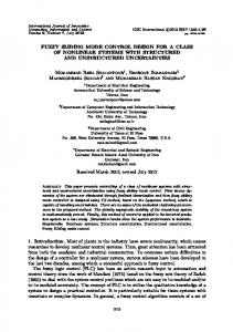
2. Mathematical model 2.1. CIPS model CIPS has two degrees of freedom, Xis the Cart displacement and θ is the pendulum angle position, as shown in Figure 1. If the cart mass is donated by M , m is the pendulum mass, L is the length between the pivot and the pendulum center of gravity C.G, g is the acceleration of gravity, I is the pendulum mass moment of inertia with respect to its C.G., Ff r is the friction force between the cart and the rail. q is the friction coefficient in the pendulum pivot. Based on D’Alembert’s principle, The equations of motion are deduced to be: ¨ + Ff r − m(Lθ¨ cos θ − Lθ˙2 sin θ) F = (M + m)X ¨ cos θ − q θ˙ (I + mL2 )θ¨ = mgL sin θ + mLX

(1) (2)

For the friction Force Ff r , most of the former work, dealing with the CIPS, either has applied a viscous friction model(linear) or has neglected its effects. However, the friction phenomena encloses many terms such as Stribeck effects, static, Coulomb and viscous frictions. Thus, exponential friction model is chosen, to address all mentioned friction parts, as follows  F X˙ ˙ s   ¯d¯  X  ¯ ˙¯  ˙   if ¯X ¯ ≤ Xd Ff r =

 n  ˙  ˙ + bX˙  FC¯ +¯(FS − FC )e−|X/VS | sgn(X)    if ¯¯X˙ ¯¯ > X˙ d

(3)

where FS is Static Friction force, FC is Coulumb Friction force, X˙ d is the dead zone velocities, VS is Stribeck velocity, n is form factor, b is the viscous friction coefficient.

Figure 1 Cart-inverted pendulum system

Appl. Math. Inf. Sci. 7, No. 1, 193-201 (2013) / www.naturalspublishing.com/Journals.asp

195

2.2. DC motor model

2.3. Overall integrated model

Figure 2. illustrates the Dc motor Circuit, where Va is the armature applied voltage (Control voltage), Vemf if the back EMF voltage, Ra , La and i are the armature resistance, inductance and current, respectively. ω is the DC Motor angular velocity, TL is the Motor electromagnetic torque, TJ is motor inertia torque, TB is the damping torque and TL is the motor load torque. The motor equations are

Here, the overall system model will be derived and the expected model will be sixth order (two coupled third equations), where the motor applied voltageVa is the system input. First, by substituting from (11),(10) and (9) in (8). And from(8) in (6) we get the current equation

Va − Vemf = i Ra + La Vemf = Ke ω

di dt

i= (4) (5)

Te Kt

(6)

Kt is the motor torque constant.Since the motor and cart move with same speed, the following equation is obtained

¨ − mLr cos θ + mLrθ¨θ˙ sin θ [(M + m)r + Jr ] + Br X di = dt Kt +2 mLr θ¨θ˙ sin θ + mLrθ˙3 cos θ + F˙f r (13) Kt

By substituting from (5),(12) and (13) in (4), we get

X˙ ω= r

(7)

J La J Ra ¨ ] ] + [[(M + m)r + ] ]X r Kt r Kt BLa ¨ BRa Ke ˙ rmLRa ¨ +[ ]X + [[ ]+[ ]]X − θ cos θ rKt r Kt r Kt rmLRa ˙2 rmLLa 3rmLLa ˙ ¨ + θ sin θ − cos θ + θθ sin θ Kt Kt Kt rmLLa ˙3 Ra La ˙ (14) + θ cos θ + Ff r + Ff r Kt Kt Kt

Va = [ [(M + m)r +

r is the motor pulley diameter.The electromagnetic torque equation will be Te = TJ + TB + TL

(8)

where TJ = J ω˙ = J TB = B ω = B TL = F r

(12)

By taking the time derivative of the last equation , (13) is obtained

Ke is the Back EMF constant. and i=

¨ ˙ ¨ + Ff r J X +B X + [(M + m)X Te r r = Kt Kt −m(L θ¨ cos θ − L θ˙2 sin θ) ]r Kt

¨ X r X˙ r

(9) (10)

This equation is considered as the main overall equation, describing the system states with the applied voltage on DC motor as an input.

(11)

From equation (2)

J is the motor rotor mass moment of inertia, B Motor rotor damping coefficient.

2 q ¨ = −g tan θ + (I + mL ) θ¨ + X θ˙ mL cos θ mL cos θ

mLg mL ¨ sin θ + cos θX (I + mL2 ) (I + mL2 ) q θ˙ − (I + mL2 )

θ¨ =

(15)

(16)

By taking the first derivative for(2) we get ... ... (I + mL2 ) θ = mgL cos θθ˙ + mLX cos θ ¨ sin θθ˙ − q θ¨ −mLX

... ¨ tan θ θ˙ + X = − g θ˙ + X

Figure 2 DC Motor circuit

... θ =

(17)

(I + mL2 ) ... q θ¨ + θ (18) mL cos θ mL cos θ

... mgL mL cos θθ˙ + X cos θ (I + mL2 ) (I + mL2 ) mL q ¨ sin θθ˙ − − X θ¨ (I + mL2 ) (I + mL2 )

(19)

c 2013 NSP ° Natural Sciences Publishing Cor.

196

Belal A.Elsayed et al : Decoupled Third-order Fuzzy Sliding ...

... Substituting from (15) and (18), with values of X and ¨ and substituting in equation (14) We get the following X, equation

¨ sin θ cos θθ˙ + f 0 cos θ sin θ ... −f 0 3 cos2 θθ˙ + f 0 4 X 5 X = [f20 cos2 θ − f10 ] ¨ + f 0 cos θθ˙ + f 0 X ¨ + f 0 X˙ +f 0 cos2 θX 6

tan θ θ˙ 2 cos θ

˙¨

θθθ ... f3 θ˙ − f4 tan2 θθ˙ + f5 tan + f6 cos θ θ = f2 ] [f1 cos θ − cos θ

¨

+ f7 cosθ θ

˙ −f8 tan θ + f9 cosθ θ + f10 X˙ − f11 θ¨ cos θ

13

f2 [f1 cos θ − cos ] θ 2 +f12 θ˙ sin θ + f13 θ˙ θ¨ sin θ + f14 θ˙3 cos θ + f15 Ff r f2 [f1 cos θ − cos ] θ +f16f r 1 − Va (20) f2 f2 [f1 cos θ − cos ] [f1 cos θ − cos ] θ θ

Where the values of constants f1→16 are [(M +m)r+ J ] La [I+mL2 ] r , Kt m L

f1 =

r m L La , Kt

f3 =

[(M +m)r+ J ] La g r , Kt

f5 =

[(M +m)r+ J ] La r Kt m L

f7 = f8 =

f2 =

f4 =

[I+mL2 ]

[(M +m)r+ J ]La g r , Kt

, f6 =

[(M +m)r+ J ] La q r , Kt m L

[

f9 = f10 = f13 =

−

14

equation(20)is the first overall system equation which will be rewritten in the form:

15

1 Va [f 0 2 cos2 θ − f 0 1 ]

(24)

0 Where the values of constants f1→15 are

f10 =

[(M +m)r+ J ]La r , Kt

f30 =

r m2 L2 La g , (I+mL2 ) Kt

f40 =

f50 =

r m2 L2 La q g (I+mL2 )2 Kt

−

f60 =

r m2 L2 La q (I+mL2 )2 Kt

f20 =

r m2 L2 Ra g (I+mL2 ) Kt r m2 L2 Ra (I+mL2 ) Kt

−

2

t

B Ra ] r Kt

r m2 L2 La (I+mL2 ) Kt

r m2 L2 La g (I+mL2 ) Kt

r m L La q f70 = − (I+mL 2 )2 K +

r m L Ra q (I+mL2 ) Kt

J Ra ] r Kt

+[

B La ]] r Kt

+ [ Kre ]]]

0 f11 =

3r m L La q r m L Ra − (I+mL 2) K Kt t 3 r m2 L2 La g 0 3 r m2 L2 La , f = 12 (I+mL2 )Kt (I+mL2 )Kt

0 f13 =

r m L La , Kt

0 f10 =

Ra a a ] + [ Kre ]], f11 = rmLR , f12 = rmLR [[ Br K Kt Kt t rmLLa Ra La 3rmLLa , f14 = Kt , f15 = Kt , f16 = Kt Kt

9

[f20 cos2 θ − f10 ]

f90 = [ [

]]q

... ˙ θ, X, ˙ θ, X, ˙ X) + β1 (θ, ˙ X) Va θ = α1 (θ,

8

f80 = [ [(M + m) r +

[(M +m)r+ J ]La q+[[(M +m)r+ J ]Ra +[ B rLa ]](I+mL2 ) r r Kt mL a a [[(M + m) r + Jr ] R + [ BL ]]g, Kt r Kt [(M +m)r+ J ]Ra +[ B rLa r Kt m L

7

[f20 cos2 θ − f10 ] ˙ 2 θ + f 0 θ˙ sin θ cos θX ¨ +f 0 10 θ˙2 sin θ + f 0 11 θsin 12 0 0 2 [f2 cos θ − f1 ] 0 3 ˙ +f θ cos θ + f 0 Ff r + f 0 F˙f r

0 f14 =

Ra , Kt

0 f15 =

La Kt

equation(24)is the second overall system equation which will be rewritten in the form:

(21)

... ˙ θ, X, ˙ θ, X, ˙ X) + β2 (θ, ˙ X)Va X = α2 (θ,

(25)

where α1 =

f3 θ˙ − f4 tan2 θθ˙ + f5

tan θ θ˙ θ¨ cos θ

[f1 cos θ −

+ f6

tan θ θ˙ 2 cos θ

¨

+ f7 cosθ θ

f2 ] cos θ

f2 [f1 cos θ − cos ] θ 2 +f12 θ˙ sin θ + f13 θ˙ θ¨ sin θ + f14 θ˙3 cos θ + f15 Ff r f2 [f1 cos θ − cos ] θ +f16f r (22) f2 [f1 cos θ − cos ] θ

1 [f1 cos θ −

f2 ] cos θ

¨ sin θ cos θθ˙ + f 0 cos θ sin θ −f 0 3 cos2 θθ˙ + f 0 4 X 5 0 [f 2 cos2 θ − f 0 1 ] ¨ + f 0 cos θθ˙ + f 0 X ¨ + f 0 X˙ +f 0 cos2 θX 6

˙ −f8 tan θ + f9 cosθ θ + f10 X˙ − f11 θ¨ cos θ

β1 = −

α2 =

(23)

7

8

9

[f 0 2 cos2 θ − f 0 1 ] 0 2 ˙ 2 θ + f 0 θ˙ sin θ cos θX ¨ +f 10 θ˙ sin θ + f 0 11 θsin 12 0 [f 2 cos2 θ − f 0 1 ] +f 0 θ˙3 cos θ + f 0 Ff r + f 0 F˙f r 13

14

15

[f 0 2 cos2 θ − f 0 1 ] β2 = −

1 Va [f 0 2 cos2 θ − f 0 1 ]

(26) (27)

3. Controller design 3.1. FSMC design

To get the second overall system ... equation, substituting from (19) and (16) with values of θ and θ¨ in equation (14)

c 2013 NSP ° Natural Sciences Publishing Cor.

In the following section, the FSMC is presented based on the derived integrated model. First, the third-order SMC is

Appl. Math. Inf. Sci. 7, No. 1, 193-201 (2013) / www.naturalspublishing.com/Journals.asp

obtained using the sliding surface concept. Next, FLC is design and applied jointly with SMC to overcome the control signal chattering. From the system equations (21) and (25) , and if D1 (t) and D2 (t) are bounded external disturbances, the entire system model will have the following form ... (28) θ = α1 + β1 Va + D1 ... X = α2 + β2 Va + D2

197

... V˙ = S1 (C1 2 θ˙ + 2C1 θ¨ + θ ) from equation 3.1 V˙ = S1 (C1 2 θ˙ + 2C1 θ¨ + α1 + β1 Va + D1 ) If the control signal Va has the following form, V˙ will be negative: Va = Vˆa −K sgn(S1 β1 ),

K>

D1 |β1 |

(35)

(29)

where 2 ˙ ¨ C1 θ−α 1 where α1 and β1 are nonlinear functions of the system Vˆa = −C1 θ−2 β1 ˙ X˙ and θ. ¨ α2 and β2 are functions of θ, X, states θ, X, θ, This form of the control signal guarantee the stability ˙ X˙ and X. ¨ θ, for the pendulum subsystem since V˙ is kept negative. In ˙ ¨ ¨ For CIPS, the system states areθ, θ, θ, X, X˙ and X.Therefore, order to ensure for the whole system stability, the intermeSMC will be used in the third-order form. The control law diate link function is introduced as follows: is designed based on the sliding surface where the system First, the first sliding surface will be reformed to be states is moved from any general position towards the sliding surface and keep sliding till the equilibrium point. S1 = C1 2 (θ − Z) + 2C1 θ˙ + θ¨ (36) The general equation for the sliding surface S is [7] based on the new sliding surface, the control target changed h iT h iT d (n−1) T T S(x, t) = ( + C) x (30) from θ θ˙ θ¨ = [0 0 0] to be θ θ˙ θ¨ = [Z 0 0] . dt Where Z is the intermediary function which is a function where x is the system sate, n is the system order and C ofS2 . The objective S2 = 0 is embedded in the main conis a constant value. In this case(CIPS) the system consists trol target through the variable which is defined to be of two third order subsystems. So that, two sliding surface S2 for the pendulum subsystem and S1 for the Cart subS2 system, are considered where Z = sat( )ZU (37) φz S1 = C1 2 θ + 2C1 θ˙ + θ¨ (31) ZU is the upper limit of the function, φz is the function boundary layer. At any general condition, the controller will move the system states θ˙ and θ¨ to zero. consequently, ¨ S2 = C2 2 X + 2C2 X˙ + X (32) the intermediate function Z converges to zero. In that case where C1 and C2 are a positive constants. Sliding surand from equation (36) and (37), it could be found that faces S1 andS2 are constructed based on the values of C1 both of S1 and S2 will be decaying to zero [14]. and C2 . Thus, the system response is highly dependent on The control action Va , as it is shown in equation (35), Values of C1 and C2, appropriate values of these constant has a high-frequencies switching because of the Sgn funcwill achieve the desired system response. tion. To overcome this problem, a bounder layer will be formed using a simple fuzzy controller. Such a kind of conBased on the sliding surfaces, the control law will be troller will be capable of reject all the high-frequencies and generated. Since only one control action is available, the solve the chattering problem. The controller equation will Pendulum angle will be considered as primary control tarbe modified to be get and the cart position is the secondary one. First, the controller is designed to achieve the primary target where Va = Vˆa − Kf uzzy (38) S1 = 0. Then, an intermediate function is used to link Kf uzzy is the fuzzy controller output. between the secondary and primary targets. This function Nine general bill type membership functions have been will achieve the cart subsystem stability if the pendulum chosen for the input (S1 B1 ) and output (Kf uzzy ). This stability is reached. type will generate a smooth curve to reject any undesired Considering Lyapunov function frequencies. As it is illustrated in Figure 3. and Figure 4., ZR is zero, NS is negative small, NB is negative big, 1 (33) V = S1 2 NVB is negative very big, PS is positive small, PM posi2 tive medium and, PB is Positive big, PVB is positive very As it is known from Lyapunov theorem, if V˙ is negabig. φ is the upper bound of the boundary layer which is an tive, that means the system will be moving to the sliding indicators for the width of boundary layers.Thus, choossurface and remains sliding till the stability is achieved ing suitable values for φ will reject any undesirable frequencies. K is the fuzzy output saturation φ and should be V˙ = S˙ 1 S1 (34) selected according to the DC motor limits

c 2013 NSP ° Natural Sciences Publishing Cor.

198

Belal A.Elsayed et al : Decoupled Third-order Fuzzy Sliding ...

The fuzzy surface is formed using the following IFTHEN rules IF (S1 B1 ) is N V B THEN (Kf uzzy ) is P V B IF (S1 B1 ) is N B THEN (Kf uzzy ) is P B IF (S1 B1 ) is N M THEN (Kf uzzy ) is P M IF (S1 B1 ) is N S THEN (Kf uzzy ) is P S IF (S1 B1 ) is ZR THEN (Kf uzzy ) is ZR IF (S1 B1 ) is P S THEN (Kf uzzy ) is N S IF (S1 B1 ) is P M THEN (Kf uzzy ) is N M IF (S1 B1 ) is P B THEN (Kf uzzy ) is N B IF (S1 B1 ) is P V B THEN (Kf uzzy ) is N V B The fuzzy controller output is shown in Figure 5. Figure 5 Fuzzy controller surface

3.2. LQRC design LQR control technique is widely used in controlling linear system. It has been applied to stabilize CIP after linearzing the state-space system equations around the pendulum angle stability position[2] [3]. In this case, the system states ˙ x3 = θ, ¨ x4 = X, are defined to be x1 = θ, x2 = θ, ˙ ¨ x5 = X and x6 = X. By approximating third order differental equations (2.21)and (2.25) around the equilibrium point where x = [0 0 0 0 0 0 0]T , the overall system linear equation is obtained. The general state-sapce form is x˙ = Ax + Bu

Figure 3 Input membership functions

(39)

where x is state matrix (1x6), u control signal matrix (1x1), A state parameters matrix (6x6), B control signal parameters matrix (1x6). Since only one control action(DC motor voltage) is available,u = Va . The equivalent state-space linearized system equation is  ˙  0 1 0 θ 0 0 1  θ¨     ...   −f8 f3 +f9 f7 −f11  θ   f1 −f2 f1 −f2 f1 −f2  = X˙   o 0 0    0 0 X ¨  0 ... f50 f70 −f30 0 X f20 −f10 f20 −f10   0  0   1   f −f  2 1 +  0  Va    0 

0 0 0 0 0 0

0 0 f10 f1 −f2

1 0

  θ   θ˙      ¨ θ     X   ˙   X 0 0 f6 +f8 ¨ X 0 0 0 0 0 0 1

f90 f20 −f10 f2 −f1

(40)

1 f10 −f20

Figure 4 Output membership function

From LQR theory, the following sate feedback control law is applied. u = Va = −Kx

c 2013 NSP ° Natural Sciences Publishing Cor.

(41)

Appl. Math. Inf. Sci. 7, No. 1, 193-201 (2013) / www.naturalspublishing.com/Journals.asp

Where K is the optimal feedback gain matrix required to get a minimum performance index J Z

∞

J=

(xT Qx + uT Ru)

199

Controller parameters must be carefully selected where all system limits should be considered. All FSMC and LQRC parameters are shown in Table 2 and Table 3, respectively.

(42)

0

Where Q and R are a real symmetric matrices which are chosen by the designer. The gain matrix K is calculated by solving Reduced-matrix Riccati equation (43), after obtaining matrix P . AT P + P A − P BR−1 B T P + Q = 0

parameter Value

C1 4.6

C2 2.2

φ 1×104

φz 19

K 15

(43)

where P is an intermediate matrix used to calculate the gain matrix K [15] K = R−1 B T P

Table 2 FSMC parameters

(44)

The controller parameter Q should be carefully chosen based on the states priority. Form a control point of view, the pendulum angle θ is much more important than the cart position X. Therefore, a bigger value should be chosen for the angle θ element in Q matrix. Selection of R matrix value depends on the control signal constrains. Based on the values of Q and R, the feedback gain matrix K is obtained.

4. Simulation results In this section, the CIP system is simulated based on equations (21) and (25). A comparison study has been carried out between the proposed FSMC and LQRC technique to stabilize the system. The cart rail limits is assumed to be X = ±0.35m and the DC motor maximum voltage is Va = ±24V . A nonlinear friction force is considered between the cart and the rail according to equation (3). However, in controller design, this force is a source of uncertainty and disturbance affecting the cart motion. All CIP parameters used in this simulation are listed in Table 1. Simulation has been done using Matlab Simulink.

Table 3 LQRC parameters parameter Q R K

Value diag [25 1 1 4 1 1] 0.02 [ 234.16 68.04 5.79 -14.14 -25.50 2.50]

Using the initial conditions θ = 0.1, θ˙ = 0, θ¨ = ¨ = 0, the response of the 0, X = 0, X˙ = 0 and X pendulum angular position using the proposed FSMC and LQRC are shown in figure 6.In spite of the nonlinear friction force, The proposed controller could reach the stability position faster than LQRC which has some oscillations around the stability position. figure 7. shows the cart position response. A reduced value of overshoot using FSMC (around 0.1 m) is observed in comparing with LQRC where the overshoot has reached 0.3 m. The LQRC response has continued to show oscillations around the zero position. The control signal response is shown in figure 8. The full stability is achieved by FSMC whereas LQRC response shows oscillations near the zero voltage.Thanks for the Fuzzy controller, all high-frequencies are eliminated in the FSMC response.

Table 1 System parameters parameter value M 0.882 kg m 0.23 kg L 0.3302 m I 7.88x 10−3 kg.m2 g 9.81 m/s2 q 0.0001 N.s/rad FS 0.2 N X˙ d 0.01 m/s n 4 B 8x10−7 N.m.s/rad

parameter value Kt 0.00767 N.m/A La 0.18x10−3 H Ra 2.6 Ohm r 6.35x10−3 m Ke 0.00767 V.s/rad J 3.9x10−7 kg.m2 FC 0.18 N VS 0.1 m/s b 2.5 N.s/m

Figure 6 Pendulum angle response

c 2013 NSP ° Natural Sciences Publishing Cor.

200

Belal A.Elsayed et al : Decoupled Third-order Fuzzy Sliding ...

Figure 7 Cart position response

Figure 9 Pendulum angular position response under disturbance

Figure 8 Control signal response

Figure 10 Cart response under disturbance

Moreover, to verify the robustness of the proposed FSMC, an external disturbance, with value of 0.05 rad (50% of the initial unstable position) and one second duration, has been applied after 20s. The pendulum and cart responses are shown in figure 9. and figure 10,,respectively. The pendulum angular response shows a faster response with FSMC and able to reject the disturbance more efficiently than LQRC. The maximum overshoot has been reduced by %100 using the FSMC. The cart response shows the robustness of the FSMC over the LQRC where the maximum overshoot increased by %300. Furthermore, in the LQRC, the cart has exceeded the rail limits. The simulation results revealed that FSMC provides faster response and better robustness comparing to LQRC under similar practical constraints.

Nonlinear friction model is added to describe the friction between the cart and the rail. A third-order FSMC is proposed to stabilize the derived CIP model. This controller guarantees the overall system stability. Chattering and all undesirable frequencies in the control signal has been eliminated by forming a boundary layer using a fuzzy controller. A third-order LQRC is also presented and compared with the proposed FSMC. Despite the system constrains and external disturbance (50% of the initial condition), simulation results of FSMC show its effectiveness and robustness over the LQRC. Using the proposed FSMC instead of LQRC has decreased the cart response overshoot by 300% and the pendulum response by %100.

5. Conclusion In this paper, two third-order differential equations have been developed to combine the CIP with its DC motor.

c 2013 NSP ° Natural Sciences Publishing Cor.

Acknowledgement The authors acknowledge the financial support by University of Malaya research grant (UMRG), under the grant No.RG118/11AET.The author is grateful to the anonymous referee for a careful checking of the details and for helpful comments that improved this paper.

Appl. Math. Inf. Sci. 7, No. 1, 193-201 (2013) / www.naturalspublishing.com/Journals.asp

References [1] El-Hawwary M.I., Elshafei A.L., Emara H.M., Fattah H.A.A., IEEE Transactions on Control Systems Technology 14,1135 (2006). [2] Debasish Chatterjee, Amit Patra and Harish K. Joglekar, Systems and Control Letters 47, 355 (2002). [3] Muskinja N. and Tovornik B., IEEE Transactions on Industrial Electronics 53, 631 (2006). [4] Hung J.Y. , Gao W. and Hung J.C., IEEE Transactions on Industrial Electronics 40, 2 (1993) [5] Byung-Jae Choi, Seong-Woo Kwak and Byung Kook Kim, Fuzzy Sets and Systems 106, 299 (1999). [6] Shi-Yuan Chen, Fang-Ming Yu and Hung-Yuan Chung, Fuzzy Sets and Systems 129, 335 (2002). [7] Sung-Woo Kim and Ju-Jang Lee, Fuzzy Sets and Systems 71, 359 (1995). [8] Ji-Chang Lo and Ya-Hui Kuo, IEEE Transactions on Fuzzy Systems 6, 426 (1998). [9] Chih-Min Lin and Yi-Jen Mon, IEEE Transactions on Control Systems Technology 13, 593 (2005). [10] Byungkook Yoo and Woonchul Ham, Fuzzy Sets and Systems 6, 315 (1998). [11] Lon-Chen Hung and Hung-Yuan Chung, Expert Systems with Applications 32, 1168 (2007). [12] Ferhun Yorgancioglu and Hasan Komurcugil, Expert Systems with Applications 37, 6764 (2010). [13] C.W. Tao, J.S. Taur, C.M. Wang and U.S. Chen, Fuzzy Sets and Systems 159, 2763 (2008). [14] H. Olsson, K. J. Astrom, C. C. de Wit, M. Gafvert and P. Lischinsky, Eur. J. Control 4, 176 (1998). [15] Katsuhiko Ogata, Modern Control Engineering ( Prentice Hall, Upper Saddle River, NJ,USA, 2002).

201

Belal A. Elsayed was born in Egypt in 1987. He received the B.S.degree in Mechatronics engineering from the Assiut University, Assiut, Egypt, in 2009. Since 2011, he has been working toward the M.S. degree from University of Malaya, Kuala Lumpur, Malaysia, where he has been involved in the research in areas of nonlinear control systems. His current research interests include areas of control, mechatronics, snensors and actuators. Mohsen AbdelNaeim Hassanis associate professor at the mechanical department, Faculty of Engineering, Assuit University, Egypt. Currently he is a visiting associate Professor at the Department of Engineering Design and Manufacture, Faculty of Engineering, UM. He graduated with Honours degree in Mechanical Engineering/ Design and production (Top Student among all departments in the Faculty of Engineering) in 1991, Egypt. He has received his Master in 1997, Egypt. He awarded the Japanese government Ph.D. scholarship in1998. In 2002 He got his PhD in information and production science (forming technology), Kyoto Institute of technology, Japan. He is a Professional Engineer registered with the Board of Engineers of Egypt, member of IMECH, UK, member of the of the Japan Society for Technology of Plasticity and member of the Egyptian Nanotechnology club member. He has published more than 30 technical articles in the field of forming and micro forming, MEMS, Piezoelectric thin Films and heart mechanics Saad Mekhilef (M07) received the B.Eng. degree in electrical engineering from the University of Setif, Setif, Algeria, in 1995, and the M.Eng.Sc.and Ph.D. Degrees in Electrical Engineering from the University of Malaya, Kuala Lumpur, Malaysia, in 1998 and 2003, respectively. He is currently a Professor in the Department of Electrical Engineering, University of Malaya. He has been actively involved in industrial consultancy, for major corporations in the power electronics projects.He is the author and coauthor of more than 100 publications in international journals and proceedings. His research interest includes power-conversion techniques, control of power converters, renewable energy, and energy efficiency.

c 2013 NSP ° Natural Sciences Publishing Cor.