Robust stability constraints for fuzzy model predictive control - Fuzzy

50

IEEE TRANSACTIONS ON FUZZY SYSTEMS, VOL. 10, NO. 1, FEBRUARY 2002

Robust Stability Constraints for Fuzzy Model Predictive Control Stanimir Mollov, Ton van den Boom, Federico Cuesta, Aníbal Ollero, and Robert Babuˇska

Abstract—This paper addresses the synthesis of a predictive controller for a nonlinear process based on a fuzzy model of the Takagi–Sugeno (T–S) type, resulting in a stable closed-loop control system. Conditions are given that guarantee closed-loop robust asymptotic stability for open-loop bounded-input–boundedoutput (BIBO) stable processes with an additive 1 -norm bounded model uncertainty. The idea is closely related to (small-gain-based) 1 -control theory, but due to the time-varying approach, the resulting robust stability constraints are less conservative. Therefore the fuzzy model is viewed as a linear time-varying system rather than a nonlinear one. The goal is to obtain constraints on the control signal and its increment that guarantee robust stability. Robust global asymptotic stability and offset-free reference tracking are guaranteed for asymptotically constant reference trajectories and disturbances. Index Terms— 1 -control theory, model predictive control (MPC), multiple-input–multiple-output (MIMO) systems, robust stability, Takagi–Sugeno (T–S) fuzzy models.

I. INTRODUCTION

M

ODEL predictive control (MPC) has been an active field of research during the last three decades, driven both by numerous successful applications of the technology [1]–[3] and by the research interests of the academia. The main reason of this success is the ability of MPC to control multivariable systems under constraints in an optimal way. In model predictive control, the control action is computed by solving an optimization problem on line in each sampling period. This is the main difference from conventional control, where a precomputed control law is employed. A major bottleneck in practical applications of MPC is obtaining a reliable prediction model. Fuzzy models of the Takagi–Sugeno (T–S) type proved to be suitable for the use in nonlinear MPC because of their ability to accurately approximate complex nonlinear systems, by combining data with prior knowledge [4]–[6]. Many applications of MPC based on fuzzy prediction models have been reported [7]–[12]. Recently, several papers appeared where different fuzzy MPC algorithms are analyzed and compared [13]–[15]. The methods discussed in these references can Manuscript received December 15, 2000; revised May 16, 2001. This research was supported in part by the FAMIMO Esprit project LTR 219 11. Also available at http://iridia.ulb.ac.be/FAMIMO S. Mollov, T. van den Boom, and R. Babuˇska are with the Systems and Control Engineering Group, Faculty ITS, Delft University of Technology, 2600 GA Delft, The Netherlands (e-mail: [email protected]; [email protected]; [email protected]). F. Cuesta and A. Ollero are with the Dipartimento Ingenieria de Sistemas y Automatica, Escuela Superior de Ingenieros, Universita de Sevilla, Camino de los Descubrimientos s/n, 41092 Seville, Spain (e-mail: [email protected]; [email protected]). Publisher Item Identifier S 1063-6706(02)01539-4.

generally be classified into two groups: (i) methods utilizing directly the fuzzy model in the optimization procedure [9], [14], [10], [15] and (ii) methods using a linearized model obtained from the fuzzy model [7], [8], [14], [16], [12]. For example, Kavzek and Skrjanc [8] extract a step-response model from the fuzzy model, whereas Abonyi et al. [12] apply Jacobian linearization. Other possibilities are to compute the control signals for the different fuzzy submodels separately and to weigh them [11], or to use only the submodel with the highest membership degree [7], [14]. The predictive controller discussed in this paper uses local linear models derived from the fuzzy model, as described in [16]. A linear model can be extracted from a T–S model at very low computational costs at a given working point or along a trajectory. The control signal is then obtained by solving a constrained quadratic program. A convergent iterative optimization scheme can be used to reduce the effect of linearization errors. Although the T–S model usually yields a reasonably accurate approximation of the process, one must keep in mind that a certain model-plant mismatch will always be present. This mismatch will not only deteriorate the control performance; it may even destabilize the closed-loop system. The availability of tools for the design of a robustly stable predictive controller is then of paramount importance. So far, this aspect of MPC has only been addressed for linear time-invariant (LTI) process models, typically by using techniques based on infinite prediction horizon [17] or end-point constraints [18], [19]. In the linear case, if no constraints are specified, the MPC controller can be expressed as an LTI controller the robustness of which can easily be analyzed. In the presence of constraints, robust stability can be guaranteed either by including an explicit contraction constraint [20] or by assuring that the criterion function is a contraction through the optimization of the maximum of the criterion function over all possible models [21], [22]. All of the above methods, however, are only valid for linear models and no general framework for predictive control based on a nonlinear model is available. The method presented in this paper is an extension of the method proposed in [23], where conditions are given that guarantee robust asymptotic stability for open-loop stable linear systems with an additive -norm bounded model uncertainty. Here, similar conditions are derived for open-loop stable nonlinear systems with an additive -norm bounded model uncertainty. Based on the uncertainty description, level and rate constraints for the control signal are derived that guarantee stability for any model-plant mismatch within the given bounds. The main contribution of the current paper is the derivation of time-varying level and rate constraints for a predictive controller based on a general (i.e., possibly nonfuzzy) nonlinear model. These constraints guarantee bounded-input–bounded-output

1063–6706/02$17.00 © 2002 IEEE

MOLLOV et al.: ROBUST STABILITY CONSTRAINTS FOR FUZZY MODEL PREDICTIVE CONTROL

(BIBO) stability for any model-plant mismatch within some given bounds. An algorithm is presented that extracts the uncertainty bounds when the nonlinear model is a fuzzy model of the T–S type. The method makes use of the fact that at each sampling instant, new measurements become available and thus linear time-varying constraints can easily be incorporated in the design. Input constraints are calculated at each sampling instant, based on a linear model extracted from the fuzzy model. The resulting constraints are similar to (small-gain-based) -control theory, but they are much less conservative as they are based on the uncertainty that actually occurs in the system, instead of the “allowed worst-case model uncertainty.” Similar ideas have also been investigated within the gainscheduling framework [24]–[26]. In gain scheduling, the nonlinear model is linearized at one or more operating points and linear design methods are applied to obtain a set of linear feedback control laws. It is well known that a parameter-varying system which is stable for fixed parameters may lose its stability in the presence of parameter variations. Shamma and Athans give sufficient conditions that guarantee that the overall gainscheduled system will retain the feedback properties of the local designs when the process model is linear parameter varying [25] or when it is nonlinear [26]. If the gain-scheduling methodology is used, however, stability can only be guaranteed for sufficiently slow parameter variations. Our approach does not impose this restriction, as the linear models are derived locally around the current operation point. The paper is organized as follows. Section II introduces the T–S fuzzy model and in Section III the problem to be solved is stated. Section IV presents the theoretical background of the method. Bounds on the model uncertainty for models of the T–S type are derived in Section V. The incorporation of the robust stability constraints in the model predictive control scheme is detailed in Section VI, which also addresses nominal and robust performance and offset-free reference tracking. In Section VII, a simulation example and a real-time example are presented to highlight the advantages and drawbacks of the proposed method. Finally, Section VIII concludes the paper.

51

where and specify the number of lagged values for the th output and the th input, respectively. The functions are parameterized as rule-based fuzzy models of the T–S type [4] is is

is is (2)

being the antecedent fuzzy sets of the th rule, with and vectors containing the consequent parameters and offsets. is the number of rules for the th output. The output is computed as the weighted average of the individual rules’ consequents (3) The degree of fulfillment of the th rule, , is obtained as the product of the membership degrees of the antecedent variables (states and inputs) in that rule (4)

III. PROBLEM STATEMENT The considered predictive controller computes an optimal control sequence with respect to the following cost function:

II. T–S FUZZY MODEL T–S fuzzy models are suitable for modeling a large class of nonlinear systems [4], [5]. Consider a multiple-input, multiple, and outoutput (MIMO) system with inputs, . This system is approximated by a collection puts, of coupled multiple-input–single-output (MISO) discrete-time fuzzy models. The MISO models are of the input–output NARX type (1) contains the current inputs and the The input vector contains the current and delayed regression vector outputs and delayed inputs

(5) Here, is the output predicted by the nonlinear fuzzy model, is the output increment, and are the output and input are the control signal and its increment, rereferences, and denotes the inner-product norm. The paramspectively, and , and , called the prediction, control and mineters imum cost horizon, respectively, define the intervals over which , and the optimization is carried out. The weights , determine the relative importance of the different terms in the cost function. The fuzzy model (1) is used to predict the process output, subject to (time-varying) level and rate constraints on the inputs and outputs (6a) (6b) (6c) (6d)

52


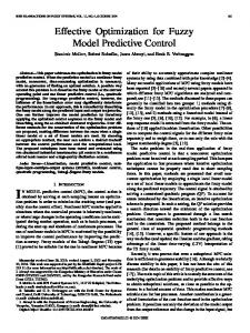
Fig. 1. Fuzzy model-based predictive control with robust stability constraints.

Due to the nonlinearity of the fuzzy model, the cost function (5) is not convex with respect to the control signal. To avoid nonconvex optimization, a single local linear model or a set of local linear models is used instead of the fuzzy model [16]. At a certain point of the predicted trajectory a local linear model is computed by linearization of the nonlinear model (Fig. 1). The resulting optimization problem has an analytic solution when no constraints are present. In the presence of constraints, quadratic programming can be used. MPC is an easy-to-tune method. In principle, there are only , three basic parameters to be tuned: the prediction horizon and the minimum control horizon , the control horizon respectively. The purpose of tuning the parameters is to obtain good reference tracking, sufficient disturbance rejection and rois the bustness against model-plant mismatch. Often best choice, but a larger value may be chosen for systems with is rea dead time or an inverse response. The choice of lated to the settling time of the process and it should capture . An important effect of the conthe crucial dynamics of is the smoothing of the control signal trol horizon ). By choosing a short (which can become very wild if , we force the control signal toward its steady-state value, which is important for stability properties. Another important is the reduction in the computaconsequence of decreasing tional effort. As an initial guess, the following settings are recommended [27]: , where is the number of pure delays from the input to the output (in samples); , where is the order of the process; • for well-damped processes, or • for poorly damped and unstable processes. is the sampling time, Here is the settling time, is the sampling frequency and is the bandwidth of the process.

•

Although a well-tuned predictive controller is usually quite robust with respect to a model-plant mismatch [28], a general theory dealing with the stability and robustness issues in predictive control is still missing. Therefore, the goal is to provide constraints on the control signal to the predictive controller that ensure stability for the closed-loop control system. Usually stability is analyzed with respect to a given process model. However, often the process is complicated and/or varies with time, hence it is impossible to obtain a perfect model. A reasonable approach is to consider the process deviation from the available model as the model uncertainty, such that the process behavior is always contained within the set of behaviors described by the model combined with the associated uncertainty. Based on the current model uncertainty, at each sample, constraints on the control signal and its increment are computed such that the control signal is in a (hyper)region where stability is guaranteed for all possible perturbations in the process. The process is considered to be linear time-varying (LTV) rather than nonlinear time-invariant (7) Denote the “true” process by available model by

, and the nominal process and (8a) (8b)

and are assumed to be bounded. The where the offsets model uncertainty , defined as the deviation of the true process from its nominal model, is then given by (Fig. 2) the equation shown at the bottom of the page. IV. DERIVATION OF THE ROBUST STABILITY CONSTRAINTS This section presents general conditions that ensure robust stability of the control system despite variations in the controlled


Fig. 3.

Feedback system for internal robust stability analysis,

!(k) + G(d(k)).

Fig. 2. A general IMC scheme which is only used to compute the stability constraints on the control signal and on its increment.

process. These conditions are valid for the class of open-loop BIBO stable processes that can be described through (7). First, some definitions for -stability are recalled [29], where the symbol stands for the Lebesque spaces. For denotes the set of all measurable functions, , , i.e., whose th powers are absolutely integrable over , while denotes the set of essentially bounded measurable functions . be an input-output mapping on . Definition IV.1: Let . Then is said to be stable if is stable with finite gain (wfg) if it is Difinition IV.2: stable, and in addition there exist finite real constants and , such that (9) is the -norm of the corresponding where signal. Remarks: 1) -stability wfg implies -stability. 2) If is an -stable wfg input-output mapping, then the -gain of is the minimal value for which there exists a nonnegative parameter , such that (9) holds: such that (9) holds . 3) The 1-norm (or the induced -norm) of is defined as (10) 4) Below BIBO stability and -stability wfg have the same meaning. Fig. 2 depicts a scheme which is used to compute the stability bounds on the control signal and its increment. It is a general two degrees-of-freedom control scheme in which all the blocks are input–output mappings. These mapping are used to obtain the signal relations that are necessary to derive the stability constraints. It is assumed that the process is described by -stable wfg , which denote the nominal model mappings and the additive model uncertainty, respectively. The mappings are the controllers to be designed. The signal is the output of the process, is the output of the feedback conis the output of the feedforward controller , which troller filters the reference trajectory , and is the output of the two de-

53

u (k)

=

grees-of-freedom controller. The signals and are additive disturbances on the input and the output of the process, respectively. Recall that is the difference between the offsets of the true , such that the parprocess and of the nominal model, allel connection of the mappings and is offset-free. To retain the input-output mapping (7), the model offset is added outside the feedback loop. It is also assumed that the model exactly represents the nominal process , i.e., the complete model-plant mismatch is contained in the additive uncertainty . . It can be seen that the Denote only feedback loop in the controlled system is the one depicted in Fig. 3. Hence, the problem of guaranteeing robust internal stability of the controlled system given in Fig. 2 can be reduced to the general problem of guaranteeing that the feedback system of Fig. 3 is robustly internally stable. In nonlinear systems, the incremental input–output mappings are different from the nonincremental ones (contrary to linear systems). Therefore, to describe the feedback system, both the incremental (denoted through ) and the nonincremental mappings are necessary

(11a)

(11b) The stability constraints proposed in [23] were derived for convolution systems (12) where the input–output mapping is a MIMO LTI system. The contains the time-invariant Markov parammatrix eters or kernels of the system [30]. The system is called causal (or ). (or strictly causal) if The following theorem gives the constraints on the controller mapping (and ) in the feedback system (11), which guarantee that this feedback system is globally internally asymptotically stable for different assumptions on and/or . Theorem IV.I: Consider the feedback system (11), where and are -stable LTI convolution operators, is strictly . Under these conditions the causal and . system is asymptotically stable if Proof: See [29, Sec. 6.6].

54


As the process model is time varying and contains the offset are term, both the uncertainty mapping and its increment time varying, and cannot be written directly in the form (12). To guarantee stability under these conditions, some necessary concepts are first introduced and then a new theorem is given. -stable with finite Assume the process model (8b) to be gain (wfg)

that is

Usually the offset is regarded as a constant [29]. However, for the sake of generality, here it may be time varying. in (11), and Thus for the uncertainty and its increment the offset it holds that and

and

The corresponding theorem states the conditions for BIBO stability of the LTV system. Theorem IV.2: Consider the feedback system (11), where and are -stable wfg LTV convolution operis strictly causal and . ators, Under these conditions, the system (11) is BIBO stable if . Proof: The proof is similar to the proof of Theorem IV.1 (see [29, Sec. 6.6]). The constraint is sufficient to guarantee stability for all possible perturbations which satisfy . However, if the true perturbation is only a small subset of all possible perturbations like, e.g., one fixed (but unknown) convolution operator, this constraint is very conservative. Less conservative stability constraints can be derived using the fact that all the signals in (11) are known up to time . Theorem IV.3: Consider the feedback system (11), where and are finite-order -stable and wfg mappings of the form (12). Further, let be causal, and be strictly causal, and and . Under these conditions the system (11) is BIBO stable if at least one of the following three constraints is satisfied. and . Ca) and Cb)

Cc)

and where and are arbitrary strictly causal -stable wfg operators of the form (12) in which the the Markov parameters (or kernels) are greater or equal to zero. and have finite orders and , and induced -norms and . which satisfy Proof: See Appendix A. Constraint Ca) is as conservative as the constraint in Theorem IV.2 and it guarantees that . Constraints Cb) and Cc) guarantee for the specific realization of the signals and that actually occur in the system. They can be less conservative than Ca), depending on the exact situation in the system. In other words, any of the constraints Ca), Cb) and Cc) guarantees stability for all possible perturbations that , but Cb) and Cc) automatically adapt satisfy , which usually to the true realization of the output of makes them less conservative [23]. The following theorems provide more easily implementable versions of the constraints Ca), Cb), and Cc). First, the constraints are defined with and since the respect to some upper bounds of actual mappings are not known. Then the current “worst-case” upper bounds and input–output disturbances are estimated. Theorem IV.4: Consider the feedback system (11), where and are operators that are -stable . Let and be causal and wfg and be strictly causal, and . Further, let and be strictly causal, finite-order -stable wfg operators of the form

or

(13)

and satisfy the following assumptions:

Define arbitrary causal -stable wfg mappings and of and . the form (13) with Then the system (11) is BIBO stable if at least one of the following two constraints is satisfied: and and

where where where mapping.

and are integers such that and , denotes the order of the corresponding

and Proof: See Appendix B.


Constraint C2) still cannot be implemented as and are unknown in practice. In the following corollary, two constraints are specified which are closely related to C2) but which can be implemented. This is achieved by using the meainstead of the nonmeasurable and/or surable signal and by using estimates of the worst-case upper bounds and . and be arbitrary strictly Corollary IV.1: Let -stable wfg mappings of the form (13) causal and . The with and can be seen as estimates of and operators at the current time instant. Then constraint C2) in Theorem IV.4 can be replaced by either of the following

and

and

Proof: See Appendix B. Remarks: • The interpretation of C3) and C4) is the same as that of Cb) and Cc). There is a close relation between C1) and Ca), but C1) can be implemented in a much simpler and computationally faster form than Ca). in Theorem IV.4 only • The true upper bounds and need to exist. If C1), C3), or C4) is used, they do not need to be known. Below we derive such bounds for the nonlinear T–S fuzzy model. V. FUZZY MODEL AS A CONVOLUTION OPERATOR The fuzzy model (1) is represented as an LTV, convolution operator of the form (12)

(17)

(18) (19) (20)

and where

then

, the fuzzy To find an expression for the kernels model is written in a specific state-space form. Since the model is assumed to match exactly the nominal process, an extended description including both the process and the model is

and where

55

-stable wfg

denotes the process state, and the model state The vector contains the regression vectors for the separate outputs in (1), reordered such that delayed outputs from all come first and then the delayed inputs. and denote the model (and The matrices in the same time the nominal process ), while the matrices and denote the real process (Fig. 2), where

(21) For the sake of notational simplicity, we drop the time argument from the state-space matrices. Given an operating point and , the state-space model is extracted as follows. according Calculate the degrees of fulfillment to (4) and define [recall (3)]

(14) is the time-varying matrix of the system’s where kernels, which will be obtained later on. To find an upper bound for the (unstructured) model uncertainty , the induced -norm is used, as it accounts for the -norms of the input and output signals (15) Recall that (Fig. 2) and (16)

The matrices and are in the standard controllable canonand positioned such that ical form with the parameters they reflect the structure of the state vector. Please see the equation shown at the bottom of the page. The model-plant mismatch is taken into account through the variations in the model parameand . These matrices have structures identers, given in tical to the ones used in and (without the ones in ), and the entries are the tripled values of the standard deviations for the corresponding parameters in the fuzzy model consequents. These parameters, together with their standard deviations, are obtained during the derivation of the fuzzy model [6].

56


Then, recall (17)

Equations (18) through (20) can be combined into (22) with

(25)

The output pansion

(maximal singular value). In order to where greater or equal to , avoid a Lyapunov transformation is introduced through a matrix , such that

can be obtained through a Volterra series ex-

(26) Then (23) Comparing (23) with (16), we obtain the needed kernels (27) To find an upper bound on the increment of the output we follow the same lines (28) .. .

Analogous to (16) and (17)

(29)

(24)

.. . .. .

..

.

..

.

.. .

.. .

..

.

.. .

..

..

.

.. .

.. .

..

.

.. .

..

.

.. .

.. .

..

.

.. .

.

.. .

.. .

.. .

.. .

.. .

.. .

.. .

..

.

..

.

.. .

.. .

..

.

..

.

.. .

..

.

..

.

.. .


57

where the matrix

is the maximal singular value and is a Lyapunov transformation, such that (and also

and

). Then (35)

VI. ROBUST FUZZY MODEL-BASED PREDICTIVE CONTROL (30) To find an expression for mental form

, we rewrite (23) in an incre-

(31) Thus

(32) with (33) where the parameters

are

.. .

This section combines the results presented so far to design a predictive controller with guaranteed robust stability for stable fuzzy models of T–S type with -bounded additive uncertainty. Both offset-free reference tracking and robust stability are guaranteed for asymptotically constant reference trajectories as ) and disturbances. The control system ( is said to be robustly stable if the process output (Fig. 2) goes when and become constant: to the constant value as and . A. Robust Stability Constrains and Uncertainty Bounds The robust stability constraints calculated through C1), C3), and the output or C4) use as parameters of the feedforward filter . Below the effect of these “tuning” parameters of the constraints is explained and guidelines are given how to select them. In practice, besides robust stability and nominal performance, robust performance is also desired. For optimal nominal perforshould be as large as posmance the constraints on and sible, while still guaranteeing stability. For robust performance should be as small as possible. the upper bounds on and Although the MPC method usually determines the compromise between the nominal and robust performance, the robust stability constraints should also influence this compromise. Nominal performance. When nominal performance is the ) could be made main objective, the constraints on (and as very loose by applying C4) and choosing large as possible. This would result in good nominal disturbance rejection. The steady-state gain of the feedforward filter should be the inverse of the steady-state gain of . Usually, the choices proposed by de Vries and van den Boom [23] and

Analogous to (25)

(36) and are much larger ensure that than the true output (and the output increment) of the model uncertainty, even if the actual model uncertainty has a different realization. For the upper bounds of the controller mappings de Vries and van den Boom suggested [23] and (34)

(37)

58


where

and and is the steady-state gain matrix of the nominal system at time instant . These choices also guarantee offset-free reference tracking. Robust performance. When robust performance is sought, can be designed in a way similar to the feedforward filter control. However, due to the LTV naLTI -control or ture of the model, has to be recomputed at each sample reflecting the current situation. In this case the constraint C1) and are computed according can be used, where to (37). This would result in conservative constraints because and and no other inforC1) only depends on and is taken into account. Such inmation about formation could be used when C3) is applied. For example, and can be chosen such that and , where and are the weighting filters used in LTI control , and is the optimal controller. B. Offset-Free Reference Tracking and Feedforward Filter Offset-free reference tracking. Although offset-free tracking should be guaranteed by the MPC method, we investigate the assumptions that the robust stability constraints must satisfy in order to make the problem (at least) feasible. must be equal to and to In steady state, , which leads to the well-known result that the steady gain of in (11) must be equal to (and ). This implies that the must be equal to in steady-state gains of and order to guarantee offset-free tracking. Hence, in steady state the are equal to . In the the1-norms of and orems given in Section IV, the condition that and must hold for each and thus also at a steady state. The latter implies that the bound on the induced -norm of the additive model uncertainty must be lower than a specific value which depends on the steady-state gain maand trix of the nominal system— . Feedforward filter. As the forward gain of the fuzzy model is not constant, the feedforward filter is recomputed at each sample. Using the optimal control sequence, computed in the previous sample, the fuzzy model is simulated over the prediction horizon, and linear models are obtained for steps . The filter gain is the inverse of the steady-state gain of these models. There are three options ; 1) a single gain based on the linear model obtained for 2) a single gain based on the entire set of linear models ; for example, the minimal of the steady-state gains; 3) different gains for every step in the prediction horizon , based on the steady-state gain of the corresponding model. While the first alternative is the simplest one, the third one leads to the most accurate calculation. The second alternative is a compromise between the two, providing a feasible solution.

Fig. 4. Two cascaded tanks setup.

The parameters in (37) are set 10% higher than the product of the uncertainty bound and the inverse of the steady-state gain of the current model, as there is an absolute upper limit of 0.9

VII. EXAMPLES A. Simulation of a SISO Liquid Level Control Process This example illustrates the computation of the uncertainty bounds, the different degree of conservatism of the three implementable constraints C1), C3) and C4), and the influence of the constraints on the performance of the controller. Consider a laboratory setup consisting of two cascaded tanks (Fig. 4). The manipulated variable is the pump flow rate and the goal is to in the lower tank such that it follows control the liquid level a prescribed reference. The fuzzy model was identified using data from the real s. The model consists process, sampled with the period of four rules of the form is is

is is

The identification technique is based on fuzzy clustering and least-squares estimation [6]. The consequent parameters and their standard variations are given in Tables I and II. The performance of the model on a validation data set is shown in Fig. 5. The variance accounted for is 90.4%. This fuzzy model is used to represent the process model in the controller. The process itself is simulated by using a perturbed fuzzy model obtained by randomly varying the consequent parameters of the original fuzzy model. The perturbed parameters . (Table III) are in the interval


59

TABLE I CONSEQUENT PARAMETERS

TABLE II STANDARD DEVIATIONS OF THE CONSEQUENT PARAMETERS

The MPC parameters are selected according to the tuning rules given in Section III. Since there is a delay of one sample, . The process is well the minimum cost horizon is used to speed-up damped and a prediction horizon of the response (the settling time is about 25 s). The process order . The weight in the cost is two, thus, control horizon is and the physical input constraints are function is . The gain of the feedforward filter (Fig. 2) is equal to the inverse of the minimal steady-state gain (second option in Section VI.B). The parameter in (36) and (37) is set , which gives a first-order filter to The calculation of the uncertainty bounds at time s is on the model uncertainty shown below. The bounds and and are computed according to (15) and (28), respectively. For the sake of illustration, the considered convolution operators in (16) and (29) are of fifth order. s, i.e., at the previous values for the lower At m and m; the tank level are and . Based control input is and extracted from on these values, the matrices the fuzzy model (23) are shown in the equation at the bottom of the page. The corresponding matrices obtained in the previous four sampling instants are

Fig. 5. Validation of the fuzzy model. Solid line: process output. Dashed line: model prediction.

TABLE III PERTURBED CONSEQUENT PARAMETERS

and the equation shown at the bottom of the next page, and the common matrix . is from (25) we have For the kernels

(38)

and using (15)–(17),

.

60


Fig. 6. Robust stability constraints C1), C3), and C4) on the control input increment q .

1

Analogously for the incremental kernels from (34) we have

(39)

and using (15) through (17), the upper bound of the uncertainty . The robust stability constraints on , is

Fig. 7. Control input increment on C1).

1q and the robust stability constraints based

computed through C1), C3) and C4) are given in Fig. 6. Since and are symmetric around zero (Theorem IV.4 is shown in the figure. The and Corollary IV.1), only input increment is secured to stay in the interval determined by and respectively (see Fig. 7 for the the bounds C1) case). Note that the constraint based on C1) is the most conservative, while the one using C4) the least conservative. The C3) constraint is between the two. After a reference change, the constraints based on C1) swiftly go to zero, while the C4) constraints allow some variation of the control signal. The C3) con-


Fig. 8. Reference tracking with (solid) and without (dashed) robust constraints.

Fig. 9. Control signal with C1) (solid) and without (dashed) robust stability constraints.

straints also tend to zero, but more slowly than the constraints based on C1). The benefits of the proposed method can be appreciated when we compare the result to unconstrained case. Figs. 8 and 9 demonstrate the difference between controllers with and without stability constraints. Without stability constraints (only are imposed) the physical constraints the system oscillates. The robust constraints smooth out the control signal, which results in a smoother output. Note that offset-free reference tracking is achieved. B. Real-Time Application to a MIMO Tank Process To demonstrate the real-time performance of the presented technique, we use a laboratory-scale cascaded-tanks process (Fig. 10). The control objective is to follow set-point changes for the levels in the lower two tanks by adjusting the flow rates of the liquid entering the upper tanks. The flow rates are the manipulated inputs and the lower levels are the controlled outputs. Coupling is introduced by cross-connecting the upper and lower tanks.

Fig. 10.

61

Four cascaded tanks setup.

Fig. 11. Validation of the fuzzy model. Top: level h . Bottom: level h . Solid line: process output. Dashed line: model prediction.

A model is obtained by using experimental input-output data, s. The structure of the model sampled with the period is defined using insight in the physical structure of the system: second-order models for both outputs with one sampling-time delay in the inputs

The performance of the model on a validation data set is shown in Fig. 11. The performance indices for the two outputs are: . The MPC parameters are selected as follows. The minimum , as in the previous section. The control cost horizon is and the prediction horizon is set only horizon is set to to improve the disturbance rejection properties. The to and . The no-zero weighting matrices are user-provided constraints on the inputs and outputs are

62


(a)

Fig. 12. Real-time control performance with and without robust stability constraints.

Two first-order Butterworth filters with the cutoff frequency Hz are used as feedback filters (see Fig. 1). The process behavior with and without robust stability constraints (C1) is presented in Fig. 12. The bounds on the control signal and its increment are not very tight, due to the existing interactions inside the model (Fig. 13). Still, the constraints on the control increment go to zero in steady-state and when no disturbances are presented. Note that since the user-provided lower bounds on the control signals are equal to zero, in Fig. 13(a) only the upper bounds are given. While in both cases the controller achieves offset-free reference tracking, the introduction of the robust stability constraints reduces the oscillations during a transition between different setpoint levels. The smoothness, however, is achieved at the exs, a temporary pense of a slightly slower response. At power failure (lasting five seconds) in the left pump was deliberately introduced. Again, the robust constraints smooth out the controller reaction to this external disturbance. However, their s when a larger deviation in conservatism appears at is observed due to a setpoint change for (Fig. 13). level

(b) Fig. 13. Robust stability constraints on the control signals and their increments.

VIII. CONCLUSION This paper presented a general scheme for computing robust stability constraints for nonlinear MPC. On the basis of -control theory, conditions have been derived that guarantee robust stability for general (also nonfuzzy) nonlinear plants. The process model is considered as a linear time-varying model, rather than a nonlinear time-invariant one, thus reducing the conservatism by computing the uncertainty bounds at each sampling instant. Based on these bounds, constraints on the control signal and its increment are calculated such that stability is guaranteed for any model-plant mismatch within the given uncertainty. A systematic procedure for the computation of the bounds on the model uncertainty has been proposed for the process model of the T–S type. The effectiveness of this approach was demonstrated through a simulated example and in real-time control of a laboratory cascaded-tanks process.


APPENDIX

Letting

63

, we get

A. Proof of Theorem IV.3 and , thus . To prove that stable wfg (BIBO stable) when Ca) is used, system (11) is consider the external signal 1) Constraint Ca): Let

Since and

and , and , we have that . In turn this implies that , and from the -stability wfg of we have that , which leads to the conclusion that the system (11) is -stable. The proof for the incremental relations proceeds along the same lines. B. Proof of Theorem IV.4 and Corollary IV.1

The above is equivalent to

The proof of Theorem IV.4 is based on the fact that upper bounds can be found that guarantee stability for all the internal and explicsignals in system (11), by analyzing itly. The proof of Corollary IV.1 is based on the same princi(or ) should be analyzed explicples, except that or itly for the case that which, together with the result C2) of Theorem IV.4, form the basis of the proof. REFERENCES

or

Since

and , and , we have that . This in turn , and from the -stability wfg of implies that we have that , which leads to the conclusion that the system (11) is -stable. The proof for the incremental relations proceeds along the same lines. 2) Constraint Cb): The constraint Cb) is a special case of (in ), corresponding to Cc) when the Markov parameter for the maximum value of is set to with . stable 3) Constraint Cc): The proof that system (11) is wfg when Cc) is used follows the same reasoning as the proof for the Ca) case and

[1] J. Richalet, “Industrial applications of model based predictive control,” Automatica, vol. 29, no. 5, pp. 1251–1274, 1993. [2] S. J. Qin and T. A. Badgwell, “An overview of industrial model predictive control technology,” in Proc. Fifth Int. Con. Chemical Process Control, 1997, pp. 232–256. [3] , “An overview of nonlinear predictive control applications,” in Nonlinear Model Predictive Control. ser. Progress in Systems and Control Theory, F. Allgöwer and A. Zheng, Eds. Boston, MA: Birkhäuser, 2000, vol. 26, pp. 369–392. [4] T. Takagi and M. Sugeno, “Fuzzy identification of systems and its application to modeling and control,” IEEE Trans. Syst., Man, Cybern., vol. 15, pp. 116–132, 1985. [5] X. J. Zeng and M. G. Singh, “Approximation theory of fuzzy systems—MIMO case,” IEEE Trans. Fuzzy Syst., vol. 3, pp. 219–235, May 1995. [6] R. Babuˇska, Fuzzy Modeling for Control. Boston, MA: Kluwer, 1998. [7] D. Saez and A. Cipriano, “Design of fuzzy model based predictive controllers and its application to an inverted pendulum,” Proc. FUZZ-IEEE, vol. 2, pp. 915–919, 1997. [8] B. K. Kavsek, D. Skrjanc, and I. Matko, “Fuzzy predictive control of a highly nonlinear pH process,” Comp. Chem. Eng., vol. 21, pp. S613–618, 1997. [9] M. Fischer, O. Nelles, and R. Isermann, “Predictive control based on local linear fuzzy models,” Int. J. Syst. Sci., vol. 29, no. 7, pp. 679–697, 1998. [10] J. Q. Hu and T. Rose, “Generalized predictive control using a neurofuzzy model,” Int. J. Syst. Sci., vol. 30, no. 1, pp. 117–122, 1999. [11] Y. L. Huang, H. H. Lou, J. P. Gong, and E. F. Thomas, “Fuzzy model predictive control,” IEEE Trans. Fuzzy Syst., vol. 8, pp. 665–678, Dec. 2000. [12] J. Abonyi, L. Nagy, and F. Szeifert, “Fuzzy model based predictive control by instantaneous linearization,” Fuzzy Sets Syst., vol. 120, no. 1, pp. 109–122, 2001. [13] J. J. Espinosa, M. L. Hadjili, V. Wertz, and J. Vandewalle, “Predictive control using fuzzy models-Comparative study,” in Proc. ECC, 1999, p. F0547. [14] H. N. Nounou and K. M. Passino, “Fuzzy model predictive control: Techniques, stability issues, and examples,” Proc. 1999 IEEE Int. Symp. Intelligent Control Intelligent Systems and Semiotics, pp. 423–428, 1999. [15] J. V. de Oliveira and J. M. Lemos, “A comparison of some adaptivepredictive fuzzy-control strategies,” IEEE Trans. Syst., Man, Cybern. C, vol. 30, pp. 138–145, Feb. 2000.

64


[16] J. A. Roubos, S. Mollov, R. Babuˇska, and H. B. Verbruggen, “Fuzzy model based predictive control by using Takagi-Sugeno fuzzy models,” Int. J. Approx. Reason., vol. 22, no. 1/2, pp. 3–30, 1999. [17] J. B. Rawlings and K. R. Muske, “The stability of constrained receding horizon control,” IEEE Trans. Automat. Contr., vol. 38, pp. 1512–1516, Oct. 1993. [18] D. W. Clarke and R. Scattolini, “Constrained receding horizon predictive control,” presented at the IEE Proc.—D, vol. 138, 1991. [19] E. Mosca and J. Zhang, “Stable redesign of predictive control,” Automatica, vol. 28, no. 6, pp. 1229–1233, 1992. [20] A. Zeng and M. Morari, “Robust Stability of Linear Systems with Constraints,” California Inst. Technol., Pasadena, CA, 1995. , “Robust stability of constrained model predictive control,” pre[21] sented at the Proc. Amer. Control Conf., 1993. , “Global stabilization of discrete-time systems with bounded [22] controls—A model predictive control approach,” presented at the Proc. Amer. Control Conf., 1994. [23] R. A. J. De Vries and T. J. J. van den Boom, “Robust stability constraints for predictive control,” presented at the Proc. ECC, vol. 6, 1997. (FR A B2). [24] W. J. Rugh, “Analytical framework for gain scheduling,” IEEE Control Syst. Mag., vol. 11, no. 1, pp. 79–84, 1991. [25] J. S. Shamma and M. Athans, “Analysis of gain scheduled control for nonlinear plants,” IEEE Trans. Automat. Contr., vol. 35, pp. 898–907, Aug. 1990. , “Guaranteed properties of gain scheduled control of linear param[26] eter-varying systems,” Automatica, vol. 27, no. 3, pp. 559–564, May 1991. [27] A. R. M. Soeterboek, Predictive Control; A Unified Approach. Upper Saddle River, NJ: Prentice-Hall, 1992. [28] J. H. Lee and Z. H. Yu, “Tuning of model predictive controllers for robust performance,” Comp. Chem. Eng., vol. 18, no. 1, pp. 15–37, 1994. [29] M. Vidyasagar, Nonlinear Systems Analysis. Upper Saddle River, NJ: Prentice Hall, 1993. [30] H. Kwakernaak and R. Sivan, Modern Signals and Systems. Upper Saddle River, NJ: Prentice-Hall, 1991.

Stanimir Mollov was born 1972 in Sliven, Bulgaria. He received the M.Sc. degree in electronics and automation engineering from the Technical University, Sofia, Bulgaria, in 1998. He is working toward the Ph.D. degree with the Systems and Control Engineering Group, the Delft University of Technology, The Netherlands. His Ph.D. project is titled “Fuzzy control of multiple-input, multiple-output processes.” His main research interests include multivariable process control, fuzzy modeling, identification, and control.

Ton van den Boom was born in Bergen op Zoom, The Netherlands. He received the M.Sc. and Ph.D. degree in electrical engineering from the Eindhoven University of Technology, The Netherlands, in 1988 and 1993, respectively. Currently, he is an Associate Professor with the Systems and Control Engineering Group at the Delft University of Technology, The Netherlands. His research interests are in the areas of nonlinear and robust model predictive control, modeling of uncertainty using fuzzy and neural models, and control of discrete-event and hybrid systems.

Federico Cuesta was born in Burgos, Spain, in 1970. He received the M.Sc. degree in computer science (with honors), and the Ph.D. degree in computer science (with doctoral award), both from the University of Seville, Spain, in 1994 and 2000, respectively. From 1993 to 1998, he was Research Assistant under several grants at the Department of Automatic Control of the University of Seville. Since 1998, he has been Assistant Professor in the same Department. His research experience includes participation in several European Projects, and stays as Researcher in the Department of Mechanics of the Technical University of Graz, Austria, the Department of Automatic Control of the Lund Institute of Technology, Sweden, and the Control Laboratory of the Delft University of Technology, The Netherlands. He is the author or coauthor of more than 30 publications including book chapters, journal papers, and conference proceedings. His current research interests include fuzzy logic, neural networks, stability analysis, nonlinear control systems, mobile robots, and teleoperation of vehicles.

Aníbal Ollero received the M.Sc. degree in electrical engineering, and the Doctor Engineer degree with doctoral award, both from the University of Seville, in 1976 and 1980, respectively. Since December 1992, he has been a Professor at the University of Seville. He has been Professor at the Universities of Santiago de Compostela in Vigo and Malaga, Spain, “stagiere” at the LABS-CARS, Toulouse, France, and Visiting Scientist at the Robotics Institute, Carnegie Mellon University, Pittsburgh, PA. He is the author or coauthor of more than 200 publications, including two books on computer control and robotics. He participated in or led 48 research and development projects funded by Spanish agencies, the European Commission, and several industries. His research activities are in new methods and technologies for robotics, perception, computer vision and intelligent control, including fuzzy control methods. He led the design and implementation of prototypes and working systems for several applications, including autonomous guidance of vehicles, forest fire detection and monitoring, teleoperation of space manipulators, and robots for greenhouse, forestry, and internal pie inspection. He is currently the Chairman of the “Manufacturing and Instrumentation” Coordinating Committee of IFAC, Associate Editor of Control Engineering Practice, and a member of the Information and Communication Technologies Committee of the Andalusian Research office. Dr. Oller is an Associate Editor of the IEEE TRANSACTIONS ON SYSTEMS, MAN, AND CYBERNETICS. His book Control por Computador: Descripció Interna y Diseño Óptimo (Marcomco Boixareu, 1991) received the Premio Mundo Electrónico Award

Robert Babuˇska received the M.Sc. degree in control engineering from the Czech Technical University, Prague, Czechoslavakia, and the Ph.D. degree from the Delft University of Technology, The Netherlands, in 1990 and 1997, respectively. Currently, he is an Associate Professor at the Systems and Control Engineering Group of the Electrical Engineering Department at the Delft University of Technology. He is an Associate Editor of Engineering Applications of Artificial Intelligence, and is an area Editor of Fuzzy Sets and Systems. He has coauthored more than 30 journal papers and chapters in books, over 100 conference papers, a research monograph entitled Fuzzy Modeling for Control (Boston, MA: Kluwer, 1998), and coedited two books. His main research interests are fuzzy set techniques and neural networks for nonlinear systems identification and control. Dr. Babuˇska is currently an Associate Editor of the IEEE TRANSACTIONS ON FUZZY SYSTEMS.