effects that commonly degrade accuracy of positioning solutions. One approach to overcome .... Cooperative TOA (CTOA) - A single BS (N = 1) obtains measurements T. (i,1] ..... [16] M.S. Grewal and A.P. Andrews. Kalman Filter: Theory and ...
Copyright Notice c
2008 IEEE. Personal use of this material is permitted. However, permission to reprint/republish this material for advertising or promotional purposes or for creating new collective works for resale or redistribution to servers or lists, or to reuse any copyrighted component of this work in other works must be obtained from the IEEE.
Decoupling Estimators in Mobile Cooperative Positioning for Heterogeneous Networks Jo˜ao Figueiras† and Simone Frattasi† and Hans-Peter Schwefel†§ †
Center for TeleInFrastruktur, Aalborg University, Denmark § Forschungszentrum Telekommunikation Wien, Austria Tel. +45 9940 8625, Fax: +45 9815 1583 Email:{jf, sf, hps}@es.aau.dk
Abstract— Positioning in wireless communications represents nowadays an important topic in the research community. The main reason is the increasing number of new location based services available on the market. Since some types of these services require accurate positioning information, research has evolved in the direction of overcoming the adverse propagation effects that commonly degrade accuracy of positioning solutions. One approach to overcome propagation effects is to consider cooperative schemes where close-by users share information regarding their links. However, due to the coexistence of numerous technologies, heterogeneity and interaction between technologies shall be regarded as an additional problem. This paper proposes and analyzes a positioning framework for cooperative schemes, which is specifically beneficial for scenarios with heterogeneous link technologies.
I. I NTRODUCTION Location information of wireless Mobile Devices (MD) is nowadays one key factor for allowing operators to exploit new applications, such as Location Based Services (LBS) [1], [2]. The quality of service for some of these LBS is strongly dependent on the accuracy of the positioning method. A typical and well-known localization system to be used in such applications is the Global Positioning System (GPS) [3]. Although its accuracy is of the order of some few meters, its usage may not be desirable in certain scenarios, since it is a demanding technology in terms of power consumption and it requires integration of additional hardware in the MDs. A potentially good candidate for providing localization in wireless networks is the class of methods that estimate location information by exploiting the communication channels [2], [4]. These solutions are based on powerful prediction and estimation algorithms that use radio-propagation models and mobility models. Generally, these methods depend on the available information concerning the channel, such as Received Signal Strength (RSS), Time of Arrival (TOA), Time Difference of Arrival (TDOA), Angle of Arrival (AOA) or combinations of these measurements [2], [4], [5], [6]. Since accuracy depends on the number of sources of observations, research has evolved into cooperative solutions where common techniques for relative positioning in sensor networks are used [7], [8]. The idea relies on additional information obtained from the short-range ad-hoc links established between nearby users. This information when combined with
978-1-4244-1722-3/08/$25.00 ©2008 IEEE.
the long-range information gives more accurate estimations for the position of each one of the cooperative users. According to previous work on cooperative mobile positioning [7], [8], [9], there is no particular attention given to the heterogeneity of the networks. In this paper, the authors design a positioning framework for cooperation that is supported on the assumption that communication networks are generally heterogeneous. In this paper, the authors propose the Two Level Kalman Filter (2LKF), a solution where relative localization of the users using peer-to-peer ad-hoc links is decoupled from the absolute localization of the same users as a group. Although the framework was designed envisaging its integration with Kalman filters, extending it to other Bayesian filtering algorithms may be possible. The 2LKF implements a decoupling of shortand long-range technologies in order to differently treat the properties of the channel observations. The main motivation is to handle the different characteristics of the positioning solutions designed for the various communication technologies present in the heterogeneous network. This approach has the advantage that it allows to handle different timing behavior of the channel measurement procedure for the short- and longrange technologies, without an increase in computational complexity. Furthermore, the approach also allows for distributed computation and for inclusion of group mobility models. II. R ELATED W ORK Traditional wireless positioning in current cellular networks combines several estimates of channel properties obtained at different BSs [2], [4], [5]. Due to the varying propagation conditions of the air interface, several approaches have been developed in order to enhance the accuracy of the positioning systems. Hybrid approaches, such as combined RSS, AOA, TOA or TDOA have been developed [6], [10], [11] in order to increase the amount of information available for each device. Another approach has been to mitigate the propagation conditions in order to consider the propagation errors in the positioning algorithms [12], [13], [14]. An alternative approach, and the one used in this paper, is the use of information from nearby MDs. Possible solutions have been inspired in the WSN context [7], [8], [9], [15]. In contrast to these approaches, this paper addresses the problem of cooperative
positioning, given that current communication networks are generally heterogeneous. III. S CENARIO D ESCRIPTION The scenario is assumed to be urban, where micro cells span over a large area so that full coverage is guaranteed. Figure 1
Fig. 1.
Schematic representation of the general scenario.
shows a schematic representation of the scenario. A total of N BSs and n MDs is considered. In an absolute coordinate system, the BSs and MDs are assumed to be positioned at respectively x[i] and x(i) , with i the index of the respective BS or MD. �T �T � � x[i] = x[i] y [i] , x(i) = x(i) y (i) (1) In eq.(1), x and y correspond to the 2D position coordinates (with straightforward extension for a 3D scenario). The MDs are assumed to be static and placed within close proximity. The MDs are equipped with two different technologies, long-range links allowing communication with the BSs and short-range links allowing communication among MDs. Two major sub scenarios are considered: • Cooperative TOA (CTOA) - A single BS (N = 1) obtains measurements T (i,1] of TOA and A(i,1] of AOA from n MDs. The MDs measure RSS samples P (i,j) from the ad-hoc links among them. • Cooperative TDOA (CTDOA) - Three BSs (N = 3) obtain measurements T (i,j] of TDOA and A(i,1] of AOA from n MDs. Similarly to the CTOA case, the MDs measure RSS samples P (i,j) . The notation T (i,j] means that the quantity T is measured in the link between MD i and BS j (note differentiation of bracket types). The notation P (i,j) is equivalent to the notation T (i,j] , though it is related to a link between 2 MDs. For both cases, the AOA measurements are exclusively obtained by BS 1 and TDOA measurements have also BS 1 as a reference. IV. T WO L EVEL K ALMAN F ILTER The proposed solution consists in decoupling relative localization, realized by using the short-range ad-hoc links, and absolute localization, realized by using the long-range cellular links. As we can see in Fig. 1 (see arrows in the figure), the relative localization is done among the several cooperative
mobiles by estimating distances between pairs of MDs, while the absolute localization is done by estimating the coordinates and orientation of the group in the cellular network. The proposed framework, alike a Bayesian filter, runs in a cyclic way, where each iteration is performed when observations are available. The framework considers the following steps: 1) Decoupling into (i) relative coordinates and (ii) center of mass coordinates. 2) Depending on whether available measurements are from short- or long-range technology: a Single iteration of a stochastic filter for estimating relative localization. b Single iteration of a stochastic filter for estimating the coordinates of the center of mass. 3) Coupling estimations of relative and center of mass coordinates in order to have absolute estimators. In case that there are measurements from a single domain, only the corresponding sub-step in step 2 is executed. In case both types of measurements are available, both sub-steps in step 2 are executed in parallel. The advantage of this feature, is that it allows short- and long-range systems to operate with different measurement rates. Figure 2 shows an operational representation of the framework. The framework is general and can be used with different kinds Previous estimation of the absolute position
xk-1(i)
Decoupling (i)rel
xk-1
Group position and orientation
Relative Position
N
Short-Range Measurements Available?
Long-Range Measurements Available?
Y Short-range Measurents
N (i)rel
xk
xk-1grp
N
Y
Relative Localization
Absolute Localization
Location Information Requested?
Location Information Requested?
Y
Long-range Measurents
N
xkgrp
Y Coupling
Current estimation of the absolute position
Fig. 2.
xk(i)
Operational representation of the proposed framework.
of stochastic filtering algorithms. As we can see in Fig. 2, the algorithm operates in the case when there is only one type of measurement (either short- or long-range measurements) and also in the case when both are available. In Fig. 2, it is
important to notice two aspects. The first one is that, if there is no request for positioning during a certain execution cycle, then the coupling is not performed. This behavior lowers the amount of computation required. The second aspect is the link between the relative and absolute positioning blocks. As it is explained in Section IV-C, this is a necessary step in order to define absolute distances between MDs and BSs. A. Decoupling and Coupling Decoupling the absolute coordinates in relative coordinates, group position, and orientation is easily done by applying a transformation of coordinates. 1) Transformation of coordinates: It is necessary to obtain the Current Transformation Matrix (CTM) that corresponds to a translation followed by a rotation of the axis. Let us assume that the absolute coordinates of MD i are defined by x(i) and from the relative coordinates by x(i)rel . Moreover, assuming Tctm as the CTM for the transformation of coordinates, the following relation can be written: � (i) � � (i)rel � x x = Tctm (2) 1 1 where the last component of the vector on the right-hand-side is added to allow transformations independent of x(i) . In order to determine Tctm , we assume that a translation equivalent to absolute position x(1) of MD 1 is followed by a rotation equivalent to the angle of the segment between MD 2 and MD 1� with respect� to the absolute coordinate system, θ = arctan y (1,2) /x(1,2) . Thus: ⎡ ⎤ x(1,2) y (1,2) ⎢ (1,2) − (1,2) 0 ⎥ ⎡ ⎤ ⎢ d ⎥ d ⎢ (1,2) ⎥ 1 0 −x(1) (1,2) ⎢ y ⎥ x ⎣ 0 1 −y (1) ⎦ Tctm = ⎢ 0 ⎥ ⎢ d(1,2) ⎥ (1,2) d 1 ⎢ ⎥ 0 0 ⎣ ⎦ 0 0 1 (3) where x(1,2) = x(2) −x(1) , y (1,2) = y (2) −y (1) and d(1,2) is the Euclidean distance between MD 1 and MD 2. Note that with this transformation of coordinates, the MD 1 is the reference, and MD 2 is on the x-axis of the relative coordinate system. 2) Decoupling of coordinates: As it is visible in Fig. 2, the decoupling implies the calculation of: (i) the relative locations of the users (x(i)rel , for user i); and (ii) the group position and orientation (xgrp ). The relative coordinates of the MDs can be obtained by using eq.(2) with the CTM of eq.(3). The coordinates and orientation �of the group �is respectively obtained by x(1) and θ = arctan y (1,2) /x(1,2) . 3) Coupling of coordinates: When performing the coupling, the absolute coordinates of the MDs are obtained by including the coordinates and orientation of the group in eq.(3) and perform the inverse calculation of eq.(2). B. Relative Localization To perform an estimation of the relative localization of the MDs, an EKF was used [16]. The choice of the filter was
made due to the fact that the system has a nonlinear nature which is not very accentuated, i.e. the linearization by itself does not introduce considerable error when compared to the noise introduced by the processes involved. In order to design the EKF, one has to primarily define the hidden process and the observable process. For the present case, the hidden process is the set of relative positions, while the observations are the measured power values between the MDs. � � � �T �T T � x(3)rel ... x(n)rel (4) xrel = x(2)rel � zrel =
P (1,2) ,
P (1,3) ,
...
P (1,n) ,
P (2,3) ,
... .. .
P (2,n) , .. .
(5) �T
P (n−1,n) Note that eq.(4) does not include the coordinates of MD 1 and the y coordinate of MD 2 due to the fact that they are 0 in the relative coordinate system. In order to reduce the state space, those 0’s where excluded. It is also important to notice that zrel in eq.(5) is a column vector. Furthermore, it is assumed that short-range links are symmetric, i.e. for each pair of MDs i and j in eq.(5) there is a single observation P (i,j) where i < j. Instead, if links where not symmetric, eq.(5) would need to be extended to consider all P (i,j) with i �= j. The second step of the design of the filter is the definition of the mobility model and the observation model for the present case. Since we have assumed static devices, the predicted state is simply equal to the previous estimation, while the observation model is defined by a propagation model such as the path loss equation: ˆxrel xrel k|k−1 = ˆ k−1
�
(i,j)rel Pˆk = α − 10β log d(i,j)
�
(6) (7)
with i < j. The subscript k|k − 1, means prediction at time k given observation until time k − 1. In eq.(7), the parameter α depends on the frequency of communication, transmission power, and antenna gains, while the parameter β is the path loss exponent. The final design issue is the definition of the process noise Q and measurement noise R as defined by the EKF [16]. It is assumed that noise components are uncorrelated, i.e. covariance error matrix Q and the observation covariance error matrix R are diagonal. Concerning the measurement noise, the standard deviation of the measurements σP2 was used in the diagonal entries of R. R = σP2 I
(8)
where the matrix I is the identity matrix with the same dimension as the observation vector in eq.(5). Although σP2 in eq.(8)
is defined based on observations, its value could be obtained from either literature, computer simulation or a pre-calibration phase. Concerning the process noise Q, we can assume it to be null, since we assume static devices. However, this approach would imply the need of a large amount of measurements to allow to ignore the additional errors introduced in the position estimation by the slow convergence of the algorithm. For this reason, a process noise adaptation method, annealing (as the one implemented by [17]), is used in order to allow faster convergence of the filter. The adaptation parameters of the method are adjusted by tuning. C. Absolute Localization In contrast to relative positioning using RSS, absolute localization has strong nonlinear behavior due to the observation model for AOA. Since measurements of AOA are related with position coordinates by an arctan function, the linearization turns out to introduce additional errors in the process estimation. For this reason, an Unscented Kalman Filter (UKF) is expected to perform better than the EKF. As in the EKF, it is necessary to define the states of the hidden process and the observable process. For absolute localization, the states to be estimated are given by: � � � �T (1,2) y grp = x(1) y (1) arctan (9) x x(1,2) For the observable process, measurements are obtained from two sources: time and angle. Thus, � �T � �T � �T (1) (n) grp (1,1] (n,1] T T = A ... A z � T(i) = T (i,1]
�T ...
T (i,N ]
(10) (11)
where for CTOA we have N = 1 while for CTDOA we have N = 3. For the definition of the motion and the observation models, we recall the assumption that MDs are assumed static, meaning that predicted state equals the previously estimated. ˆgrp ˆ xgrp k|k−1 = xk−1
(12)
The observation model is given by two different expressions, one for the AOA, � � (i) [1] − y y ˆ A(i,1] = arctan (13) x ˆ(i) − x[1] and for TOA and TDOA, respectively: T (i,1] = cd(i,1] � � T (i,j] = c d(i,j] − d(i,1]
(14) (15)
Thereby, d(i,j] is the distance between MD i and BS j. It is important to notice that from eq.(13) to eq.(15), the position for MD i is obtained from xgrp and the relative distances among MDs, assuming (in absolute localization)
these distances as fixed parameters. This step corresponds to the arrow between relative and absolute localization block in Fig. 2. Concerning the covariance error matrix Q, it is modeled based on the same approach as in Section IV-B. The observation covariance error matrix R is given by: � � 2 0 σT I (16) R= 2 0 σA I 2 are standard deviations of the measurements where σT2 and σA of time and angle for the CTOA and CTDOA respectively. The matrix I is the identity matrix of adequate dimension.
D. Properties of the filter The decoupling and further coupling of the position estimator has advantages with respect to the following aspects: 1) Different observation rates: Positioning solutions generally operate with different measurement rates depending on the technology. Since it is common that long- and short-range communications are realized by different technologies, their integration in terms of positioning data requires attention. The problem is addressed with the decoupling of position estimators, which allows the two domains of data sources to operate independently (see Fig. 2). 2) Computational effort and distributed computing: Given the structure of the proposed solution, the computational effort of processing is at most as large as a framework where all measurements are equally treated [15]. Additionally, due to the decoupling of the estimators, distributed computation is possible to a certain extent. For instance short-range relative positioning can be performed by the mobile users, while longrange absolute positioning can be performed in the network. Then, depending on where the information is requested, the necessary exchange of data is performed. 3) Group mobility: The decoupling of short- and longrange domain of measurements permits the use of group mobility models. This way, the cooperative mobile users can be viewed, on one hand, as a group with correlated mobility patterns, and on the other hand, as individuals characterized by some uncorrelated mobility within the group. The consequence of such approach is that management of clusters is required when devices move out of range of their short-range links. V. P ERFORMANCE OF THE P ROPOSED S OLUTION For analyzing the performance of the 2LKF, the same simulation as the ones in [15] were implemented in order to get the measurements mentioned in Section III. In [15], longrange links model non-line-of-sight probability and excess delay, while short-range links model path loss, shadowing and fast fading. The Root Mean Square Error (RMSE) was evaluated for both CTOA and CTDOA scenarios with n = {2, 4, 6, 8, 10} cooperative MDs. The micro √ cells were 3, 1)km and simulated with 1km range placed at (0, 0), ( √ ( 3, −1)km. The center of the cluster of n MDs is assumed to be 500m apart from the main BS 1 and about 1.58km from the other BSs. The other MDs (apart of MD 1) are uniformly
1 0.9 0.8 0.7 0.6 0.5 0.4 0.3 0.2 0.1 0 0
Empirical CDF
Empirical CDF
distributed within the cluster with 25m of range around MD 1. The simulation was ran 5000 times for each value n. For each run, there were 200 measurements available from each source of measurements. For CTOA positioning, one BS was simulated while for the CTDOA, 3 BSs have been simulated. The CDF of the RMSE, plotted in Fig. 3, shows a major
non Coop 2MDs 4MDs 6MDs 8MDs 10MDs 100
200 RMSE (m)
300
400
1 0.9 0.8 0.7 0.6 0.5 0.4 0.3 0.2 0.1 0 0
non Coop 2MDs 4MDs 6MDs 8MDs 10MDs 100
200 RMSE (m)
300
400
Fig. 3. Empirical CDF of the RMSE metric for the CTOA (left) and CTDOA (right) localization technique, when the proposed 2LKF is used for data fusion.
difference concerning the cooperative case when n equals 2. In general, Fig. 3 shows that the higher the number of cooperative MDs, the higher is the accuracy. The second set of results regards the gain of the proposed approach with respect to the non-cooperative scenario. In order to simulate a non-cooperative scenario, the same absolute positioning (disregarding orientation), as in Section IV-C, was implemented for a single mobile device. The gain for the a% percentile is defined as: Ga =
c znc a − za znc a
(17)
40
20 2 MDs 4 MDs 6 MDs 8 MDs 10 MDs
0
−20 CTOA
CTDOA
Cooperation Gain for the 95%
Cooperation Gain for the 67%
where zca and znc a are the inverse CDF of the RMSE (from Fig. 3) for the percentile a% respectively in the cooperative and non-cooperative case. Figure 4 shows that there is generally 60 40 20 0
2 MDs 4 MDs 6 MDs 8 MDs 10 MDs
−20 −40 −60
CTOA
CTDOAA
Fig. 4. Gain of the 2LKF cooperative framework with respect to the noncooperative method for 67% (left) and 95% (right) of all the tested cases
a gain in accuracy when cooperation is used. However, for the case of n = 2, there may be a loss of accuracy, what results from the fact that the adverse propagation conditions are hardly overcome by only 2 cooperative MDs. When the number od cooperative MDs increases, this problem tends to be solved. VI. C ONCLUSIONS AND F UTURE W ORK This paper proposes and analyzes a positioning framework for cooperative schemes, which is specifically beneficial for scenarios with heterogeneous link technologies. This framework has the advantage that it allows to handle different timing behavior of the channel measurement procedure for
the short- and long-range technologies, without an increase in computational complexity. Furthermore, the approach also allows for distributed computation and for inclusion of group mobility models. This cooperative solution shows enhancements of accuracy when using more than two cooperative devices in comparison to non-cooperative approaches. As the proposed approach requires some form of cluster management, future work will investigate the interaction of cluster-formation algorithms with the positioning approach in dynamic settings. ACKNOWLEDGMENTS Parts of this research have been supported by the Danish Ministry of Science, Technology and Innovation in the WANDA innovation consortium and by the ICT project ICT-217033 WHERE, which is partly funded by the European Union. R EFERENCES [1] A. K¨upper. Location-based services. Wiley, 2005. [2] A.H. Sayed, A. Tarighat, and N. Khajehnouri. Network-based wireless location: challenges faced in developing techniques for accurate wireless location information. IEEE Signal Processing Magazine, 22:24–40, July 2005. [3] E.D. Kaplan et al. Understanding GPS: Principles and Applications. Artech House, 1996. [4] M. Vossiek, L. Wiebking, P. Gulden, J. Wieghardt, and C. Hoffmann. Wireless local positioning - concepts, solutions, applications. In Proceedings of Radio and Wireless Conference, 2003. RAWCON ’03, pages 219–224, August 2003. [5] F. Gustafsson and F. Gunnarsson. Mobile positioning using wireless networks: possibilities and fundamental limitations based on available wireless network measurements. IEEE Signal Processing Magazine, 22:41–53, July 2005. [6] M. McGuire, K.N. Plataniotis, and A.N. Venetsanopoulos. Data fusion of power and time measurements for mobile terminal location. IEEE Transactions on Mobile Computing, 4(2):142–153, 2005. [7] C. Mayorga, F. Rosa, S. Wardana, G. Simone, M. Raynal, J. Figueiras, and S. Frattasi. Cooperative Positioning Techniques for Mobile Localization in 4G Cellular Networks. In Proceedings of the IEEE International Conference on Pervasive Services (ICPS 2007), pages 39–44, July 2007. [8] S. Frattasi, M. Monti, and R. Prasad. Cooperative Mobile User Location for Next-Generation Wireless Cellular Networks. In Proceedings of IEEE International Conference on Communications, 2006. ICC ’06, volume 12, pages 5760–5765, 2006. [9] Q. Cui, J. Liu, X. Tao, and P. Zhang. A Novel Location Model for 4G Mobile Communication Networks. In Proceedings of the 66th IEEE Vehicular Technology Conference, 2007. VTC-2007 Fall, pages 274–278, 2007. [10] P. Deng and P.Z. Fan. An AOA assisted TOA positioning system. volume 2, pages 1501–1504, 2000. [11] L. Cong and W. Zhuang. Hybrid TDOA/AOA mobile user location for wideband CDMA cellular systems. IEEE Trans. Wirel. Commun., 1:439–447, 2002. [12] L. Cong and W. Zhuang. Non-line-of-sight error mitigation in TDOA mobile location. In Proceedings of the IEEE Global Telecommunications Conference, 2001. GLOBECOM’01, volume 1, pages 680–684, 2001. [13] P. Deng and P.Z. Fan. An efficient position-based dynamic location algorithm. In Proceedings of the 2000 International Workshop on Autonomous Decentralized Systems, pages 36–39, 2000. [14] N.R. Yousef and A.H. Sayed. Adaptive multipath resolving for wireless location systems. In Proceedings of the 2000 International Workshop on Autonomous Decentralized Systems, volume 2, pages 36–39, 2000. [15] S. Frattasi and J. Figueiras. Ad-Coop Positioning System : Using an Embedded Kalman Filter Data Fusion, pages 120–131. CRC Press, 2007. [16] M.S. Grewal and A.P. Andrews. Kalman Filter: Theory and Practice Using MATLAB. John Wiley & Sons, 2 edition, 2001. [17] R.V. Merwe and E.A. Wan. Rebel: Recursive bayesian estimation library. MATLAB library, October 2006.