Deep adversarial neural decoding

Ya˘gmur Güçlütürk*, Umut Güçlü*, Katja Seeliger, Sander Bosch, Rob van Lier, Marcel van Gerven, Radboud University, Donders Institute for Brain, Cognition and Behaviour Nijmegen, the Netherlands [f]irst.[pre][last]@donders.ru.nl *Equal contribution

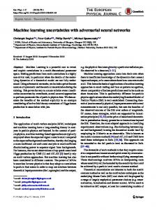
Abstract Here, we present a novel approach to solve the problem of reconstructing perceived stimuli from brain responses by combining probabilistic inference with deep learning. Our approach first inverts the linear transformation from latent features to brain responses with maximum a posteriori estimation and then inverts the nonlinear transformation from perceived stimuli to latent features with adversarial training of convolutional neural networks. We test our approach with a functional magnetic resonance imaging experiment and show that it can generate state-of-the-art reconstructions of perceived faces from brain activations.

ConvNet (adversarial training)

likelihood (Gaussian)

posterior (Gaussian) maximum a posteriori

brain resp.

ConvNet (pretrained) + PCA

prior (Gaussian)

latent feat.

*reconstruction *from brain resp. perceived stim.

arXiv:1705.07109v1 [q-bio.NC] 19 May 2017

Deep adversarial neural decoding

Figure 1: An illustration of our approach to solve the problem of reconstructing perceived stimuli from brain responses by combining probabilistic inference with deep learning.

1

Introduction

A key objective in sensory neuroscience is to characterize the relationship between perceived stimuli and brain responses. This relationship can be studied with neural encoding and neural decoding in functional magnetic resonance imaging (fMRI) [1]. The goal of neural encoding is to predict brain responses to perceived stimuli [2]. Conversely, the goal of neural decoding is to classify [3, 4], identify [5, 6] or reconstruct [7–10] perceived stimuli from brain responses. The recent integration of deep learning into neural encoding has been a very successful endeavor [11, 12]. To date, the most accurate predictions of brain responses to perceived stimuli have been achieved with convolutional neural networks [13–19], leading to novel insights about the functional organization of neural representations. At the same time, the use of deep learning as the basis for neural decoding has received less widespread attention. Deep neural networks have been used for classifying or identifying stimuli via the use of a deep encoding model [15] or by predicting intermediate stimulus features [20, 21]. Deep belief networks and convolutional neural networks have been used to reconstruct basic stimuli (handwritten characters and geometric figures) from patterns of

brain activity [22, 23]. However, to date, it has not been shown that complex naturalistic stimuli can be reconstructed with high accuracy. The integration of deep learning into neural decoding is an exciting approach for solving the reconstruction problem, which is defined as the inversion of the (non)linear transformation from perceived stimuli to brain responses to obtain a reconstruction of the original stimulus from patterns of brain activity alone. Reconstruction can be formulated as an inference problem, which can be solved by maximum a posteriori estimation. Multiple variants of this formulation have been proposed in the literature [24–29]. At the same time, significant improvements are to be expected from deep neural decoding given the success of deep learning in solving image reconstruction problems in computer vision such as colorization [30], face hallucination[31], inpainting [32] and super-resolution [33]. Here, we present a new approach by combining probabilistic inference with deep learning, which we refer to as deep adversarial neural decoding (DAND). Our approach first inverts the linear transformation from latent features to observed responses with maximum a posteriori estimation. Next, it inverts the nonlinear transformation from perceived stimuli to latent features with adversarial training and convolutional neural networks. An illustration of our model is provided in Figure 1. We show that our approach achieves state-of-the-art reconstructions of perceived faces from the human brain.

2 2.1

Methods Problem statement

Let x ∈ Rh×w×c , z ∈ Rp , y ∈ Rq be a stimulus, feature, response triplet, and φ : Rh×w×c → Rp be a latent feature model such that z = φ(x) and x = φ−1 (z). Without loss of generality, we assume that all of the variables are normalized to have zero mean and unit variance. We are interested in solving the problem of reconstructing perceived stimuli from brain responses: ˆ = φ−1 (arg max Pr (z | y)) x

(1)

z

where Pr(z | y) is the posterior. We reformulate the posterior through Bayes’ theorem:   ˆ = φ−1 arg max [Pr(y | z) Pr(z)] x

(2)

z

where Pr(y | z) is the likelihood, and Pr(z) is the prior. In the following subsections, we define the latent feature model, the likelihood and the prior. 2.2

Latent feature model

We define the latent feature model φ(x) by modifying the VGG-Face pretrained model [34]. The model is a 16-layer convolutional neural network, which was trained for face recognition. We retain the first 14 layers and discard the last two layers of the model. At this point, the model outputs 4096-dimensional latent features. Then, we combine the model with principal component analysis. That is, we estimate the loadings that project the 4096-dimensional latent features to the first 699 principal component scores and add them at the end of the model as a new fully-connected layer. At this point, the model outputs 699-dimensional latent features. Following the ideas presented in [35–37], we define the inverse of the feature model φ−1 (z) (i.e., the image generator) as a convolutional neural network which transforms the 699-dimensional latent variables to 64 × 64 × 3 images and estimate its parameters via an adversarial process. The generator comprises five deconvolution layers: The ith layer has 210−i kernels with a size of 4 × 4, a stride of 2 × 2, a padding of 1 × 1, batch normalization and rectified linear units. Exceptions are the first layer which has a stride of 1 × 1, and no padding; and the last layer which has three kernels, no batch normalization [38] and hyperbolic tangent units. Note that we do use the inverse of the loadings in the generator. To enable adversarial training, we define a discriminator (ψ) along with the generator. The discriminator comprises four convolution layers. The ith layer has 25+i kernels with a size of 4 × 4, a stride of 2 × 2, a padding of 1 × 1, batch normalization and leaky rectified linear units with a slope of 0.2 2

except for the first layer which has no batch normalization and last layer which has one kernel, a stride of 1 × 1, no padding, no batch normalization and a sigmoid unit. We train the generator and the discriminator by pitting them against each other in a two-player zero-sum game, where the goal of the discriminator is to discriminate stimuli from reconstructions and the goal of the generator is to generate reconstructions that are indiscriminable from original stimuli. This ensures that reconstructed stimuli are similar to target stimuli on a pixel level and a feature level. The discriminator is trained by iteratively minimizing the following discriminator loss function:   Ldis = −E log(ψ(x)) + log(1 − ψ(φ−1 (z))) (3) where ψ is the output of the discriminator which gives the probability that its input is an original stimulus and not a reconstructed stimulus. The generator is trained by iteratively minimizing a generator loss function, which is a linear combination of an adversarial loss function, a feature loss function and a stimulus loss function:   Lgen = −λadv E log(ψ(φ−1 (z))) +λfea E[kξ(x) − ξ(φ−1 (z))k2 ] +λsti E[kx − φ−1 (z)k2 ] (4) | {z } | {z } | {z } Lfea

Ladv

Lsti

where ξ is the relu3_3 outputs of the pretrained VGG-16 model [39, 40]. 2.3

Likelihood and prior

We define the likelihood as a multivariate Gaussian distribution over y: Pr(y|z) = Ny (B> z, Σ)

(5)

where B = (β 1 , . . . , β q ) ∈ Rp×q and Σ = diag(σ12 , . . . , σq2 ) ∈ Rq×q . We estimate the parameters ˆ = arg min E[kyi − β > zk2 ] and σ ˆ > zk2 ]. with ordinary least squares, such that β ˆ 2 = E[kyi − β i

βi

i

i

i

We define the prior as a zero mean and unit variance multivariate Gaussian distribution Pr(z) = Nz (0, I). 2.4

Posterior

To derive the posterior (2), we first reformulate the likelihood as a multivariate Gaussian distribution over z:   1 > −1 1 > > −1 > > −1 > > Ny (B z, Σ) ∝ exp − y Σ y + y Σ B z − (B z) Σ B z 2 2  1 > −1 = exp − y B BΣ−1 B> (B> )−1 y + z> BΣ−1 B> (B> )−1 y 2 (6)  1 > − z BΣ−1 B> z 2
> −1 > −1 −1 ∝ Nz (B ) y, (B ) ΣB This allows us to write: Pr(z|y) ∝ Nz (B> )−1 y, (B> )−1 ΣB−1 )Nz (0, I




(7)

Next, recall that the product of two multivariate Gaussians can be formulated in terms of one multivariate Gaussian [41]. That is, Nz (m1 , Σ1 )Nz (m2 , Σ2 ) ∝ Nz (mc , Σc ) with mc =


−1 −1 −1 −1 −1 Σ−1 Σ−1 m1 + Σ−1 . By plugging this formula1 + Σ2 2 m2 and Σc = Σ1 + Σ2 tion into Equation (7), we obtain Pr(z|y) ∝ Nz (mc , Σc ) with 3

(8)

mc = (BΣ−1 B> + I)−1 BΣ−1 y and Σc = (BΣ−1 B> + I)−1 . Recall that we are interested in reconstructing stimuli from responses by generating reconstructions from the features that maximize the posterior. Notice that the (unnormalized) posterior is maximized at its mean mc since this corresponds to the mode for a multivariate Gaussian distribution. Therefore, the solution of the problem of reconstructing stimuli from responses reduces to the following simple expression:
ˆ = φ−1 (BΣ−1 B> + I)−1 BΣ−1 y x (9)

3 3.1

Results Datasets

We used the following datasets in our experiments: fMRI dataset. We collected a new fMRI dataset, which comprises face stimuli and associated bloodoxygen-level dependent (BOLD) responses. The stimuli used in the fMRI experiment were drawn from [42–44] and other online sources, and consisted of photographs of front-facing individuals with neutral expressions. We measured BOLD responses (TR = 1.4 s, voxel size = 2 × 2 × 2 mm3 , whole-brain coverage) of two healthy adult subjects (S1: 28-year old female; S2: 39-year old male) as they were fixating on a target (0.6 × 0.6 degree) [45] superimposed on the stimuli (15 × 15 degrees). Each face was presented at 5 Hz for 1.4 s and followed by a middle gray background presented for 2.8 s. In total, 700 faces were presented twice (for a training set), and 48 faces were repeated 13 times for a test set. The experiment was approved by the local ethics committee (CMO Regio Arnhem-Nijmegen) and the subjects provided written informed consent in accordance with the Declaration of Helsinki. Our fMRI dataset will be shared online post publication. The stimuli were preprocessed as follows: Each image was cropped and resized to 224 × 224 pixels. This procedure was organized such that the distance between the top of the image and the vertical center of the eyes was 87 pixels, the distance between the vertical center of the eyes and the vertical center of the mouth was 75 pixels, the distance between the vertical center of the mouth and the bottom of the image was 61 pixels, and the horizontal center of the eyes and the mouth was at the horizontal center of the image. The fMRI data were preprocessed as follows: Functional scans were realigned to the first functional scan and the mean functional scan, respectively. Realigned functional scans were slice time corrected. Anatomical scans were coregistered to the mean functional scan. Brains were extracted from the coregistered anatomical scans. Finally, stimulus-specific responses were deconvolved from the realigned and slice time corrected functional scans with a general linear model [46]. CelebA dataset [47]. This dataset was used for adversarial training. It comprises 202599 in-the-wild portraits of 10177 people, which were drawn from online sources. The portraits are annotated with 40 attributes and five landmarks. We preprocessed the portraits as we preprocessed the stimuli in our fMRI dataset. 3.2

Implementation details

Our implementation makes use of Chainer and Cupy with CUDA and cuDNN [48] except for the following: The VGG-16 and VGG-Face pretrained models were ported to Chainer from Caffe [49]. Principal component analysis was implemented in scikit-learn [50]. fMRI preprocessing was implemented in SPM [51]. Brain extraction was implemented in FSL [52]. We trained the discriminator and the generator on the entire CelebA dataset by iteratively minimizing the discriminator loss function and the generator loss function in sequence for 100 epochs with Adam [53]. Model parameters were initialized as follows: biases were set to zero, the scaling parameters were drawn from N (1, 2·10−2 I), the shifting parameters were set to zero and the weights were drawn from N (1, 10−2 I) [36]. We set the hyperparameters of the loss functions as follows: λadv = 102 , λdis = 102 , λfea = 10−2 and λsti = 2 · 10−6 [37]. We set the hyperparameters of the optimizer as follows: α = 0.001, β1 = 0.9, β2 = 0.999 and  = 108 [36]. We estimated the parameters of the likelihood term on the training split of our fMRI dataset. 4

3.3

Evaluation metrics

We evaluated our approach on the test split of our fMRI dataset with the following metrics: First, the feature similarity between the stimuli and their reconstructions, where the feature similarity is defined as the Euclidean similarity between the features, defined as the relu7 outputs of the VGGFace pretrained model. Second, the Pearson correlation coefficient between the stimuli and their reconstructions. Third, the structural similarity between the stimuli and their reconstructions [54]. All evaluation was done on a held-out set not used at any point during model estimation or training.

3.4

Reconstruction

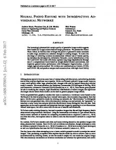
We first demonstrate our results by reconstructing the stimulus images in the test set using i) the latent features and ii) the brain responses. Figure 2 shows 16 representative examples of the test stimuli and their reconstructions. The first column of both panels show the original test stimuli. The second column of both panels show the reconstructions of these stimuli x from the latent features z obtained by φ(x). These can be considered as an upper limit for the reconstruction accuracy of the brain responses since they are the best possible reconstructions that we can expect to achieve with a perfect neural decoder that can exactly predict the latent features from brain responses. The third and fourth columns of the figure show reconstructions of brain responses to stimuli of Subject 1 and Subject 2, respectively.

stim.

reconstruction from: model brain 1 brain 2

stim.

reconstruction from: model brain 1 brain 2

Figure 2: Reconstructions of the test stimuli from the latent features (model) and the brain responses of the two subjects (brain 1 and brain 2). Visual inspection of the reconstructions from brain responses reveals that they match the test stimuli in several key aspects, such as gender, skin color and facial features. Furthermore, reconstruction accuracy for both subjects were significantly above chance level (p  0.05, permutation test). Table 1 shows three reconstruction accuracy metrics for both subjects in terms of the ratio of the reconstruction accuracy from the latent features to the reconstruction accuracy from brain responses. 5

Table 1: Reconstruction accuracy of the proposed decoding approach. The results are reported as the ratio of accuracy of reconstructing from brain responses and latent features.

S1 S2

3.5

Feature similarity

Pearson correlation coefficient

Structural similarity

0.6546 ± 0.0220 0.6465 ± 0.0222

0.6512 ± 0.0493 0.6580 ± 0.0480

0.8365 ± 0.0239 0.8325 ± 0.0229

Interpolation and sampling

In the second experiment, we first investigated the model representations to better understand what kind of features drive the model’s responses. We visualized the features explaining the highest variance by setting the values of the first few features to vary between their minimum and maximum values (Figure 3). As a result, we found that many of the latent features were coding for interpretable high level information such as age, gender, etc. For example, the first feature in Figure 3 appears to code for gender, the second one appears to code for hair color and complexion, the third one appears to code for age, and the fourth one appears to code for two different facial expressions. reconstruction (from features) feature i = min. feature i = max.

stim.

reconstruction (from features) feature i = min. feature i = max.

4

3

feature

2

1

stim.

Figure 3: Reconstructions from features with single features set to vary between their minimum and maximum values. We then explored the feature space that was learned by the latent feature model and the response space that was learned by the likelihood by systematically traversing the reconstructions obtained from different points in these spaces. Figure 4A shows examples of reconstructions of stimuli from the latent features (rows one and four) and brain responses (rows two, three, five and six), as well as reconstructions from their interpolations between two points (columns three to nine). The reconstructions from the interpolations between two points show semantic changes with no sharp transitions. Figure 4B shows reconstructions from latent features sampled from the model prior (first row) and from responses sampled from the response prior of each subject (second and third rows). The reconstructions from sampled representations are diverse and of high quality. These results provide evidence that no memorization took place and the models learned relevant and interesting representations [36]. Furthermore, these results suggest that neural representations of faces might be embedded in a continuous and distributed space in the brain. 3.6

Comparison with state of the art

In this section we qualitatively (Figure 5) and quantitatively (Table 2) compare the performance of our approach with two existing decoding approaches from the literature. Figure 5 shows example reconstructions from brain responses with three different approaches, namely with our approach, the eigenfaces approach [29] and the identity transform approach [55, 27]. To achieve a fair comparison, the implementations of the three approaches only differed in terms of the feature models that were 6

A

recon.

recon. (from interpolated features or responses)

recon.

stim.

brain 2 brain 1

reconstruction from: model brain 2 brain 1

model

stim.

B reconstruction from: brain 2 brain 1 model

recon. (from sampled features or responses)

Figure 4: Reconstructions from interpolated (A) and sampled (B) latent features (model) and brain responses of the two subjects (brain 1 and brain 2).

used, i.e. the eigenfaces approach had an eigenfaces (PCA) feature model and the identity transform approach had simply an identity transformation in place of the feature model. Visual inspection of the reconstructions displayed in Figure 5 shows that DAND clearly outperforms the existing approaches. In particular, our reconstructions better capture the features of the stimuli such as gender, skin color and facial features. Furthermore, our reconstructions are more detailed, sharper, less noisy and more photorealistic than the eigenfaces and identity transform approaches. A quantitative comparison of the performance of the three approaches shows that the reconstruction accuracies achieved by our approach were significantly higher than those achieved by the existing approaches (p  0.05, Student’s t-test). Table 2: Reconstruction accuracies of the three decoding approaches.

Identity Eigenface DAND

Feature similarity

Pearson correlation coefficient

Structural similarity

S1 S2 S1 S2

0.1254 ± 0.0031 0.1254 ± 0.0038 0.1475 ± 0.0043 0.1457 ± 0.0043

0.4194 ± 0.0347 0.4299 ± 0.0350 0.3779 ± 0.0403 0.2241 ± 0.0435

0.3744 ± 0.0083 0.3877 ± 0.0083 0.3735 ± 0.0102 0.3671 ± 0.0113

S1 S2

0.1900 ± 0.0052 0.1867 ± 0.0054

0.4679 ± 0.0358 0.4722 ± 0.0344

0.4662 ± 0.0126 0.4676 ± 0.0130

7

deep recon. eigen. recon. identity recon. from: from: from: stim. brain 1 brain 2 brain 1 brain 2 brain 1 brain 2

Figure 5: Reconstructions from brain responses of the two subjects (brain 1 and brain 2) using our decoding approach, as well as the eigenface and identity transform approaches for comparison.

3.7

Factors contributing to reconstruction accuracy

Finally, we investigated the factors contributing to the quality of reconstructions from brain responses. All of the faces in the test set had been annotated with 30 objective physical measures (such as nose width, face length, etc.) and 14 subjective measures (such as attractiveness, gender, ethnicity, etc.). Among these measures, we identified five subjective measures that are important for face perception [56–61] as measures of interest and supplemented them with an additional measure of stimulus complexity. Complexity was included because of its important role in visual perception [62]. The selected measures were attractiveness, complexity, ethnicity, femininity, masculinity and prototypicality. Note that the complexity measure was not part of the dataset annotations and was defined as the Kolmogorov complexity of the stimuli, which was taken to be their compressed file sizes [63]. To this end, we correlated the reconstruction accuracies of the 48 stimuli in the test set (for both subjects) with their corresponding measures (except for ethnicity) and used a two-tailed Student’s t-test to test if the multiple comparison corrected (Bonferroni correction) p-value was less than the critical value of 0.05. In the case of ethnicity we used one-way analysis of variance to compare the reconstruction accuracies of faces with different ethnicities. We were able to reject the null hypothesis for the measures complexity, femininity and masculinity, but failed to do so for attractiveness, ethnicity and prototypicality. Specifically, we observed a significant negative correlation (r = -0.3067) between stimulus complexity and reconstruction accuracy. Furthermore, we found that masculinity and reconstruction accuracy were significantly positively correlated (r = 0.3841). Complementing this result, we found a negative correlation (r = -0.3961) between femininity and reconstruction accuracy. We found no effect of attractiveness, ethnicity and prototypicality on the quality of reconstructions. 8

4

Conclusion

In this study we combined probabilistic inference with deep learning to derive a novel deep neural decoding approach. We tested our approach by reconstructing face stimuli from BOLD responses at an unprecedented level of accuracy and detail, matching the target stimuli in several key aspects such as gender, skin color and facial features as well as identifying several perceptual factors contributing to the reconstruction accuracy. Deep decoding approaches such as the one developed here are expected to play an important role in the development of new neuroprosthetic devices that operate by reading subjective information from the human brain.

References [1] T. Naselaris, K. N. Kay, S. Nishimoto, and J. L. Gallant, “Encoding and decoding in fMRI,” NeuroImage, vol. 56, no. 2, pp. 400–410, may 2011. [2] M. van Gerven, “A primer on encoding models in sensory neuroscience,” J. Math. Psychol., vol. 76, no. B, pp. 172–183, 2017. [3] J. V. Haxby, “Distributed and overlapping representations of faces and objects in ventral temporal cortex,” Science, vol. 293, no. 5539, pp. 2425–2430, sep 2001. [4] Y. Kamitani and F. Tong, “Decoding the visual and subjective contents of the human brain,” Nature Neuroscience, vol. 8, no. 5, pp. 679–685, apr 2005. [5] T. M. Mitchell, S. V. Shinkareva, A. Carlson, K.-M. Chang, V. L. Malave, R. A. Mason, and M. A. Just, “Predicting human brain activity associated with the meanings of nouns,” Science, vol. 320, no. 5880, pp. 1191–1195, may 2008. [6] K. N. Kay, T. Naselaris, R. J. Prenger, and J. L. Gallant, “Identifying natural images from human brain activity,” Nature, vol. 452, no. 7185, pp. 352–355, mar 2008. [7] B. Thirion, E. Duchesnay, E. Hubbard, J. Dubois, J.-B. Poline, D. Lebihan, and S. Dehaene, “Inverse retinotopy: Inferring the visual content of images from brain activation patterns,” NeuroImage, vol. 33, no. 4, pp. 1104–1116, dec 2006. [8] Y. Miyawaki, H. Uchida, O. Yamashita, M. aki Sato, Y. Morito, H. C. Tanabe, N. Sadato, and Y. Kamitani, “Visual image reconstruction from human brain activity using a combination of multiscale local image decoders,” Neuron, vol. 60, no. 5, pp. 915–929, dec 2008. [9] T. Naselaris, R. J. Prenger, K. N. Kay, M. Oliver, and J. L. Gallant, “Bayesian reconstruction of natural images from human brain activity,” Neuron, vol. 63, no. 6, pp. 902–915, sep 2009. [10] S. Nishimoto, A. T. Vu, T. Naselaris, Y. Benjamini, B. Yu, and J. L. Gallant, “Reconstructing visual experiences from brain activity evoked by natural movies,” Current Biology, vol. 21, no. 19, pp. 1641–1646, oct 2011. [11] D. L. K. Yamins and J. J. Dicarlo, “Using goal-driven deep learning models to understand sensory cortex,” Nat. Neurosci., vol. 19, pp. 356–365, 2016. [12] N. Kriegeskorte, “Deep neural networks: A new framework for modeling biological vision and brain information processing,” Annu. Rev. Vis. Sci., vol. 1, no. 1, pp. 417–446, 2015. [13] D. L. K. Yamins, H. Hong, C. F. Cadieu, E. A. Solomon, D. Seibert, and J. J. DiCarlo, “Performance-optimized hierarchical models predict neural responses in higher visual cortex,” Proceedings of the National Academy of Sciences, vol. 111, no. 23, pp. 8619–8624, may 2014. [14] S.-M. Khaligh-Razavi and N. Kriegeskorte, “Deep supervised, but not unsupervised, models may explain IT cortical representation,” PLoS Computational Biology, vol. 10, no. 11, p. e1003915, nov 2014. [15] U. Güçlü and M. van Gerven, “Deep neural networks reveal a gradient in the complexity of neural representations across the ventral stream,” Journal of Neuroscience, vol. 35, no. 27, pp. 10 005–10 014, jul 2015. [16] U. Güçlü and M. van Gerven, “Increasingly complex representations of natural movies across the dorsal stream are shared between subjects,” NeuroImage, vol. 145, pp. 329–336, jan 2017.

9

[17] R. M. Cichy, A. Khosla, D. Pantazis, A. Torralba, and A. Oliva, “Comparison of deep neural networks to spatio-temporal cortical dynamics of human visual object recognition reveals hierarchical correspondence,” Scientific Reports, vol. 6, no. 1, jun 2016. [18] U. Güçlü, J. Thielen, M. Hanke, and M. van Gerven, “Brains on beats,” in Advances in Neural Information Processing Systems, 2016. [19] M. Eickenberg, A. Gramfort, G. Varoquaux, and B. Thirion, “Seeing it all: Convolutional network layers map the function of the human visual system,” NeuroImage, vol. 152, pp. 184–194, may 2017. [20] T. Horikawa and Y. Kamitani, “Generic decoding of seen and imagined objects using hierarchical visual features,” CoRR, vol. abs/1510.06479, 2015. [21] ——, “Hierarchical neural representation of dreamed objects revealed by brain decoding with deep neural network features,” Frontiers in Computational Neuroscience, vol. 11, jan 2017. [22] M. van Gerven, F. de Lange, and T. Heskes, “Neural decoding with hierarchical generative models,” Neural Comput., vol. 22, no. 12, pp. 3127–3142, 2010. [23] C. Du, C. Du, and H. He, “Sharing deep generative representation for perceived image reconstruction from human brain activity,” vol. arXiv:1704, pp. 1–9, 2017. [24] B. Thirion, E. Duchesnay, E. Hubbard, J. Dubois, J.-B. Poline, D. Lebihan, and S. Dehaene, “Inverse retinotopy: inferring the visual content of images from brain activation patterns,” Neuroimage, vol. 33, no. 4, pp. 1104–1116, 2006. [25] T. Naselaris, R. J. Prenger, K. N. Kay, M. Oliver, and J. L. Gallant, “Bayesian reconstruction of natural images from human brain activity,” Neuron, vol. 63, no. 6, pp. 902–915, 2009. [26] U. Güçlü and M. van Gerven, “Unsupervised learning of features for Bayesian decoding in functional magnetic resonance imaging,” in Belgian-Dutch Conference on Machine Learning, 2013. [27] S. Schoenmakers, M. Barth, T. Heskes, and M. van Gerven, “Linear reconstruction of perceived images from human brain activity,” NeuroImage, vol. 83, pp. 951–961, dec 2013. [28] S. Schoenmakers, U. Güçlü, M. van Gerven, and T. Heskes, “Gaussian mixture models and semantic gating improve reconstructions from human brain activity,” Frontiers in Computational Neuroscience, vol. 8, jan 2015. [29] A. S. Cowen, M. M. Chun, and B. A. Kuhl, “Neural portraits of perception: Reconstructing face images from evoked brain activity,” NeuroImage, vol. 94, pp. 12–22, jul 2014. [30] R. Zhang, P. Isola, and A. A. Efros, “Colorful image colorization,” Lect. Notes Comput. Sci., vol. 9907 LNCS, pp. 649–666, 2016. [31] Y. Güçlütürk, U. Güçlü, R. van Lier, and M. van Gerven, “Convolutional sketch inversion,” in Lecture Notes in Computer Science. Springer International Publishing, 2016, pp. 810–824. [32] D. Pathak, P. Krähenbühl, J. Donahue, T. Darrell, and A. A. Efros, “Context encoders: Feature learning by inpainting,” CoRR, vol. abs/1604.07379, 2016. [33] C. Ledig, L. Theis, F. Huszar, J. Caballero, A. P. Aitken, A. Tejani, J. Totz, Z. Wang, and W. Shi, “Photo-realistic single image super-resolution using a generative adversarial network,” CoRR, vol. abs/1609.04802, 2016. [34] O. M. Parkhi, A. Vedaldi, and A. Zisserman, “Deep face recognition,” in British Machine Vision Conference, jul 2016. [35] I. J. Goodfellow, J. Pouget-Abadie, M. Mirza, B. Xu, D. Warde-Farley, S. Ozair, A. C. Courville, and Y. Bengio, “Generative adversarial networks,” CoRR, vol. abs/1406.2661, 2014. [36] A. Radford, L. Metz, and S. Chintala, “Unsupervised representation learning with deep convolutional generative adversarial networks,” CoRR, vol. abs/1511.06434, 2015. [37] A. Dosovitskiy and T. Brox, “Generating images with perceptual similarity metrics based on deep networks,” CoRR, vol. abs/1602.02644, 2016. [38] S. Ioffe and C. Szegedy, “Batch normalization: Accelerating deep network training by reducing internal covariate shift,” CoRR, vol. abs/1502.03167, 2015.

10

[39] K. Simonyan and A. Zisserman, “Very deep convolutional networks for large-scale image recognition,” CoRR, vol. abs/1409.1556, 2014. [40] J. Johnson, A. Alahi, and F. Li, “Perceptual losses for real-time style transfer and super-resolution,” CoRR, vol. abs/1603.08155, 2016. [41] K. B. Petersen and M. S. Pedersen, “The matrix cookbook,” nov 2012, version 20121115. [42] D. S. Ma, J. Correll, and B. Wittenbrink, “The Chicago face database: A free stimulus set of faces and norming data,” Behavior Research Methods, vol. 47, no. 4, pp. 1122–1135, jan 2015. [43] N. Strohminger, K. Gray, V. Chituc, J. Heffner, C. Schein, and T. B. Heagins, “The MR2: A multi-racial, mega-resolution database of facial stimuli,” Behavior Research Methods, vol. 48, no. 3, pp. 1197–1204, aug 2015. [44] O. Langner, R. Dotsch, G. Bijlstra, D. H. J. Wigboldus, S. T. Hawk, and A. van Knippenberg, “Presentation and validation of the Radboud faces database,” Cognition & Emotion, vol. 24, no. 8, pp. 1377–1388, dec 2010. [45] L. Thaler, A. Schütz, M. Goodale, and K. Gegenfurtner, “What is the best fixation target? the effect of target shape on stability of fixational eye movements,” Vision Research, vol. 76, pp. 31–42, jan 2013. [46] J. A. Mumford, B. O. Turner, F. G. Ashby, and R. A. Poldrack, “Deconvolving BOLD activation in event-related designs for multivoxel pattern classification analyses,” NeuroImage, vol. 59, no. 3, pp. 2636–2643, feb 2012. [47] Z. Liu, P. Luo, X. Wang, and X. Tang, “Deep learning face attributes in the wild,” in Proceedings of International Conference on Computer Vision (ICCV), 2015. [48] S. Tokui, K. Oono, S. Hido, and J. Clayton, “Chainer: a next-generation open source framework for deep learning,” in Advances in Neural Information Processing Systems Workshops, 2015. [49] Y. Jia, E. Shelhamer, J. Donahue, S. Karayev, J. Long, R. B. Girshick, S. Guadarrama, and T. Darrell, “Caffe: Convolutional architecture for fast feature embedding,” CoRR, vol. abs/1408.5093, 2014. [50] F. Pedregosa, G. Varoquaux, A. Gramfort, V. Michel, B. Thirion, O. Grisel, M. Blondel, P. Prettenhofer, R. Weiss, V. Dubourg, J. Vanderplas, A. Passos, D. Cournapeau, M. Brucher, M. Perrot, and E. Duchesnay, “Scikit-learn: Machine learning in Python,” Journal of Machine Learning Research, vol. 12, pp. 2825–2830, 2011. [51] K. Friston, J. Ashburner, S. Kiebel, T. Nichols, and W. Penny, Eds., Statistical Parametric Mapping: The Analysis of Functional Brain Images. Academic Press, 2007. [52] M. Jenkinson, C. F. Beckmann, T. E. Behrens, M. W. Woolrich, and S. M. Smith, “FSL,” NeuroImage, vol. 62, no. 2, pp. 782–790, aug 2012. [53] D. P. Kingma and J. Ba, “Adam: A method for stochastic optimization,” CoRR, vol. abs/1412.6980, 2014. [54] Z. Wang, A. Bovik, H. Sheikh, and E. Simoncelli, “Image quality assessment: From error visibility to structural similarity,” IEEE Transactions on Image Processing, vol. 13, no. 4, pp. 600–612, apr 2004. [55] M. van Gerven and T. Heskes, “A linear gaussian framework for decoding of perceived images,” in 2012 Second International Workshop on Pattern Recognition in NeuroImaging. IEEE, jul 2012. [56] A. C. Hahn and D. I. Perrett, “Neural and behavioral responses to attractiveness in adult and infant faces,” Neuroscience & Biobehavioral Reviews, vol. 46, pp. 591–603, oct 2014. [57] D. I. Perrett, K. A. May, and S. Yoshikawa, “Facial shape and judgements of female attractiveness,” Nature, vol. 368, no. 6468, pp. 239–242, mar 1994. [58] B. Birkás, M. Dzhelyova, B. Lábadi, T. Bereczkei, and D. I. Perrett, “Cross-cultural perception of trustworthiness: The effect of ethnicity features on evaluation of faces’ observed trustworthiness across four samples,” Personality and Individual Differences, vol. 69, pp. 56–61, oct 2014. [59] M. A. Strom, L. A. Zebrowitz, S. Zhang, P. M. Bronstad, and H. K. Lee, “Skin and bones: The contribution of skin tone and facial structure to racial prototypicality ratings,” PLoS ONE, vol. 7, no. 7, p. e41193, jul 2012. [60] A. C. Little, B. C. Jones, D. R. Feinberg, and D. I. Perrett, “Men’s strategic preferences for femininity in female faces,” British Journal of Psychology, vol. 105, no. 3, pp. 364–381, jun 2013.

11

[61] M. de Lurdes Carrito, I. M. B. dos Santos, C. E. Lefevre, R. D. Whitehead, C. F. da Silva, and D. I. Perrett, “The role of sexually dimorphic skin colour and shape in attractiveness of male faces,” Evolution and Human Behavior, vol. 37, no. 2, pp. 125–133, mar 2016. [62] Y. Güçlütürk, R. H. A. H. Jacobs, and R. van Lier, “Liking versus complexity: Decomposing the inverted U-curve,” Frontiers in Human Neuroscience, vol. 10, mar 2016. [63] D. Donderi and S. McFadden, “Compressed file length predicts search time and errors on visual displays,” Displays, vol. 26, no. 2, pp. 71–78, apr 2005.

12