Dec 15, 1989 - gray-level difference, Fourier Power Spectrum, Auto Correlation, etc. .... using a training set containing known samples from each of the k .... In many industrial applications (e.g. uniformity of paint finish on automotive bodies), ...
Computers & Elect. Engng Vol. 16, No. 2, pp. 65-77, 1990 Printed in Great Britain. All rights reserved
TEXTURE
0045-7906/90 $3.00 + 0.00 Copyright © 1990 Pergamon Press plc
IN IMAGES:
COMPARISON
AND
ALGORITHMS
FOR
SEGMENTATION
REN LIANG l, M . SHRIDHAR I a n d M . AHMADI 2 )Department of Electrical and Computer Engineering, University of Michigan-Dearborn, Dearborn, MI 48128, U.S.A. and 2Department of Electrical Engineering, University of Windsor, Windsor, Ontario, Canada N9B 3P4
(Received 15 December 1989; received for publication 1 February 1990) A b s t r a c t - - The extraction of features that are sensitive to texture in an image has been the subject of
intensive investigations in recent years. Recently, several important industrial applications based on the texture of a surface or texture in a scene have been identified. Many of these applications involve classification of texture, comparison of two texture samples or segmentation of an image into texturally homogenous regions. In this paper, the maximum likelihood technique has been adopted to enable comparison of two textures (similarity measure) as well as segmentation of a given image into texturally homogenous regions. In addition, features are derived from the gradient of the image rather than the spatial gray-level co-occurence matrix. A new measure of similarlity termed, "the similarity index (SI)" has been derived for comparing two textures (e.g. homogeneity of a painted surface). Experimental results with a variety of textures have demonstrated the feasibility of the new approaches taken.
1. I N T R O D U C T I O N In many important applications involving image analysis, it is frequently required to segment a given image into homogeneous regions. Such homogeneous regions are characterized by invariant features within the segment. Many papers have recently appeared in literature [1-5] that provide techniques for segmenting an image based on such criteria as homogeneity of gray level, edge detection and tracking, thresholding etc. Many of these techniques are essentially point (pixel) operations, in that, they assign a single pixel to a given region based on its location, gray level and/or gradient. However, these techniques are not generally suitable if the given image is characterized by texture. Such images can arise when an object is imaged on a textured background or if the image itself consists of one or more textures. Applications include analysis of aerial scenes (landsat pictures), SAR data and characterization of shape of textured objects. Several new techniques[6-11] have been proposed for automatic classification of texture whereby the texture in a scene (or part of a scene) is assigned to one of a finite number of known texture classes. In this paper the authors present a new measure termed, "the similarity index", for comparing these textures. Also the authors use the "gradient histogram" feature developed by Raafat and Wong [7] and the gray-level co-occurrence matrix proposed by Haralick [8] for the development of a general algorithm that can; (i) classify a texture sample as belonging to one of several prespecified classes (ii) yield a measure of similarity (or dissimilarity) when two textures are compared (iii) segment a given textured image into texturally homogenous regions. Tests done with a variety of textures and textured images have shown that the alogorithm yields satisfactory classification, comparison or segmentation. 2. T E X T U R E S S E N S I T I V E F E A T U R E S Many different types of features have been proposed for measurement and characterization of texture. Some of these include the gray-level co-occurrence matrix, the gray-level run-length, gray-level difference, Fourier Power Spectrum, Auto Correlation, etc. [8,11]. Of the many features available, the gray-level co-occurrence matrix has been widely used by many investigators. The advantage of using the co-occurrence matrix lies in the fact that several 65
REN LIANGet al.
66
sub-features such as angular second moment, correlation, contrast, entropy, etc. can be derived for obtaining a unique characterization of a given texture. Recently some investigators notably Derin, Elliott et al. [15,16], have used Markov Random Field characterization for textural scenes. In this interesting approach, the authors have used a hierarchical Gibbsian model to characterize texture in terms of a finite number of parameters. Although, techniques for the estimation of these texture parameters were suggested, the authors in their study simply assumed that these parameters were known a priori. It is felt that this assumption, coupled with the computational complexity of their algorithms could be restrictive for certain applications. However this is a promising area for further developments. Other studies by Raafat [7], Weszka et al. [12] have indicated that the gradient of the image can be used to derive features that are sensitive to texture. Further the features based on gradient could be made sensitive to the orientation of texture characteristics by retaining the directional information. A final point here, is that the gradients may be evaluated efficiently. The texture-sensitive feature is derived as a gradient histogram. The feature is derived as follows: Given an image array f ( i , j), the directional gradients G, and G~ are computed as
G,.(i,j) = [f(i + l, j -[f(i-
1, j -
1) + 2 f l ( i + l , j ) + f ( i + 1 , j + 1)] 1) + 2 f ( i - 1,j) + f ( i -
1, j + 1)]
(1)
G,(i, j ) = [f(i - 1, j - 1) + 2f(i, j - 1) + f ( i + 1, j - 1)]
-[f(i-
1,j + 1) + 2f(i, j + 1) + f ( i + 1,j + 1)].
(2)
The gradient magnitude and direction are computed as
G(i, j ) = G~.(i, j ) + G~(i, j )
(3a)
O(i, j ) = tan ' (G,./G,.).
(3b)
The gradient histogram is derived by coding the magnitude and direction. In this study the magnitude is quantized to N~ levels and the direction is quantized to N2 levels as shown in Fig. l(a). Ignoring the region with zero magnitude one obtains a total of N 2 ( N 1 - - l ) levels. Thus any gradient value can be mapped into one of the N 2 ( N 1 -- 1) levels. The frequency distribution of the mapped levels in a given textured image is derived as a histogram g(n) corresponding the level n[1 ~< n ~< N 2 ( N I - 1 ) ] . The author used 13 levels for magnitude and 8 levels for direction (i.e. N~ = 13, N2 = 8) in this study Fig. 1. The characterization of texture in terms of gradient function is not a new concept; Weszka et al. [12] have in their work indicated that local properties such as gray-level and gradients are very useful in characterizing texture. A typical texture set and its quantized version and gradient along with the histogram are shown in Fig. 1 (b,c). 3. T H E
MAXIMUM
LIKELIHOOD
TECHNIQUE
FOR TEXTURE
In this section, the derivation of the maximum likelihood function for texture classification, will be presented. The derivation is similar to the technique proposed by Vickers and Modestino [6]. The major difference, in this paper, lies in the use of gradient histogram as the feature instead of the co-occurrence matrix used by Vickers and Modestino. The classification is made based on the maximum value of the likelihood function with respect to the texture classes. The derivation proceeds as follows: Let Lk(g) be the likelihood function for the texture class k where k is in (0, K - 1), the g is the gradient histogram vector. Lk(g) is defined as L~(g) = ln[P(glk)],
k = 0, 1, 2 . . . . . K - 1
where P ( g [ k ) is the conditional probability density of the vector g given that the texture class is k (see Appendix A).
Texture in images
67
(a)
~ 0 (i)
8
3 / 3~8
S
1
-
- 5~8
91
89 ( i i i )
93~
95
Fig. 1. (a,b) Caption on p. 69.
3~8
(ii)
68
REy LIANG el al.
Fig. 1. (c,d) Caption on facing page.
Texture in images
69
Fig. 1. (a) Gradient Histogram region. (i) magnitude region. (ii) Direction region. (iii) Histogram region. (b) A texture set. (c) Quantized and equalized image of Fig. l(b). (d) gradient image of Fig. l(b). (e) Gradient histogram of a texture sample.
Given Lk(g), the classification is made as follows: Assign texture to class k 0 if
Lko(g) = max Lk (g). k
While the classification technique is simple and follows traditional lines, the major difficulty in using this approach is the need to know a priori, the conditional probability density function P {g]k }. It should be noted P {glk } is a multi-dimensional density function since g is a vector with N2(N~- 1) elements. It is shown in Appendix A, that under suitable assumptions P { g l k } can be written as P{g[k} =
g(i) L i=0
!
[Qi(k)] gu)/g(i)!
(4)
i=0
where Qi(k) is the probability o f observing ith entry in g under the assumption that the texture class is k. An underlying assumption in this derivation implies that all entries in g are assigned independently. Using the above equation in the expression for Lk(g) and ignoring terms that do not depend on k, one obtains a modified likelihood function. N
1
£k(g) = ~ g(i)ln[Qi(k)]; i=0
where N
=
N 2
(Ni -- 1).
k = 0, 1. . . . , K - - 1
(5)
70
REN L1ANG et al.
It is now only necessary to estimate Qi(k) to perform the classification. Qi(k) is estimated by using a training set containing known samples from each of the k texture classes. It can be shown that an estimate of Qe(k) is obtained as
Q~(k) = gk(i
gk(i) = gk(i)/G
(6)
i=
where G is a constant and gk(i) is the histogram of kth reference texture and g(i) is the histogram of the test texture. The likelihood function £k(g) is now redefined as N-I
£k (g) = ~ g(i)In {gk (i)/G }.
(7)
i=0
The use of this likelihood function in texture discrimination is discussed in the following section. 4. T E X T U R E S :
COMPARISON
AND SEGMENTATION
The classification of texture samples using the maximum likelihood function is a fairly simple and straightforward procedure, once Qi(k) is available. However, in many problems, it is often necessary to deal with two other applications. These are (i) Texture Comparison Given a reference texture and a test texture, it is often required to obtain a measure of similarity between the two textures. (ii) Segmentation Given an image with several different but unknown textures, it is required to segment the image into texturally homogenous regions. It is clear that both of these problems cannot be directly solved by the maximum likelihood technique. In order to solve the comparison problem, it would be desirable to define similarity measure (preferably in the range 0 1) that can be used to infer the closeness of two texture samples.
4.1. Similarity measure .for texture comparison The similarity measure for comparing two textures is derived from the likelihood function of equation (7), i.e. N-I
£k(g) = ~ g(i)ln[gk(i)/G] i=0
where g(i) represents the features of the texture image and gk(i) represents the features of the kth reference texture. £k(g) can be rewritten as £k(g) = y g(i)[In gk ( i ) - in G] = Y, g(i)In gk(i)-- Y. g(i)In G.
(8)
Observing that the second expression on the right of equation (8) is independent of k, one can define a new likelihood measure as follows C~(g) = ~ g(i) In gk(i).
(9)
An examination of equation (9) reveals that this modified likelihood measure can be effectively used to compare two textures. In fact this measure will now be used in deriving a "similarity measure" as follows: (1) Define C,,,,, = ~. g,,(i)ln[g,(i)] i
where m and n represent two texture classes.
(10)
Texture in images
71
(2) Define a "Similarity Index" Stun as
sin. =
¥
J
(11)
The motivation for this derivation is based on the following observations: (1) C,,, defined above is in fact a likelihood measure. Hence it will reach a maximum value, only when the two textures are identical (m = n) (2) Since, in any practical situation Cm, 4: C,m it is necessary to define a similarity measure that will be independent of which texture is considered as reference, i.e. one needs a measure Sin, which satisfies
Sin,,----S,m. The definition according to equation (11) satisfies this requirement. The above coefficient has its value in the range 0-1. When the two textures are identical Stun assumes the value 1. The parameter I is chosen according to the sensitivity and resolution needed, in a specific application. The authors typically used / = 10 for all the texture images in their study.
4.2. Segmentation of textured images The segmentation of a given image (consisting of multiple textures) into texturally homogenous regions can be easily achieved with the use of the new similarity index defined in the previous section. The segmentation procedure is based on the region growing technique originally proposed by the authors [13]. While the region growing technique assigned individual pixels to a region being grown based on some similarity measure, the modified technique assigns subregions of predetermined size to a texturally homogenous region being grown. The procedure consists of: (a) Starting at the Northwest corner of the given digitized image, select two adjacent subregions (i.e. textures in two adjacent windows). Please note that depending on the resolution needed in segmentation, the two windows may overlap. The region closest to the Northwest corner will be assigned a label "1"
Fig. 2. An image with multiple texture.
72
REN LIANG et al.
(b) Determine the similarity index defined in equation (11) to evaluate the similarity between the two subregions~ If the similarity index is greater than some c, assign the current label to the adjacent subregion. (c) Select the next adjacent window and repeat step (b). If no adjacent region has a similarity index greater than c, then initiate the growth of a new region with a new label by starting with an unlabelled subregion (window). (d) Continue until all subregions (windows) have been labelled. The full details of this segmentation technique may be found in [13]. 5. T E S T R E S U L T S The techniques presented in the earlier sections were implemented on a variety of textured images. The images ranged from those found in Brodatz [14] to images of painted car body surfaces supplied by Diffracto Ltd of Windsor, Canada. The following tests were performed: (1) Classification using the similarity coefficient (2) Evaluation of texture homogenity across an image (3) Segmentation of textured images.
5. I. Classification with similarity index In this approach, the sample test texture is compared with each of the reference textures and the similarity coefficients evaluated. The test texture is then identified as belonging to that reference which yields the highest similarity coefficient. If the highest similarity coefficient is less than 0.7, the test image is labelled as "unknown texture" and rejected. The results of this approach were applied to 20 textured images taken from the pages D5, D9, D14, D18, D20, D22, D27, D28, D34, D36, D52, D55, D56, D65, D66, D80, D81, D103, and D i l l of the [14]. Using the similarity index measures, the following textures among the 20 test samples used were grouped as belonging to the same class. (1) (2) (3) (4)
Textures Textures Textures Textures
of of of of
pages pages pages pages
D22 and D36. D80 and D81. D23 and D27. D5 and D28. Table I. Similarity based classification
Test/Class/ Sample 10,10 50,0 0,65 180,10 180,100 140,50 30,180 100,180 70,140
10, 10
50,0
0,65
1 1 l
1 I 1
I 1 1
180, 10
180, 100
140, 50
2 2 2
2 2 2
2 2 2
30, 180
100, 180
70, 140
3 3 3
3 3 3
3 3 3
Table 2. Similarity Index (SI) with n = 10 Texture (I) Similarity Tex (1)
10, 10 50, 0 0, 65
Tex (2)
180, 10 180, 100 140, 50
Tex
30, 180 100, 180 70, 140
(3)
Texture (2)
Texture (3)
10, 10
50,0
0,65
180, l0
180, 100
140, 50
30, 180
100, 180
70, 140
1.000
0.921 1.000
0.901 0.937 1.000
0.596 0.634 0.555
0.555 0.607 0.537
0.592 0.626 0.549
0.431 0.405 0.376
0.423 0.383 0.352
0.386 0.366 0.340
1.000
0.910 1.000
0.958 0.937 1.000
0.258 0.219 0.264
0.326 0.244 0.303
0.296 0.233 0.273
1.000
0.911 1.000
0.924 0.934 1.000
Texture in images
73
Fig. 3. (a) Painting picture set. A painted sheet metal surface (b) Another sample of painted sheet metal surface. In the authors opinion, these results are consistent with the visual interpretation of the different textures. In another study, the multiple texture image shown in Fig. 2 was used for classification. The results obtained are shown in Table 2. The rectangular windows seen in Fig. 2 represent the sample textures. The results of Table 2 clearly indicate that the sample textures were correctly classified. 5.2. Texture homogeneity in an image In m a n y industrial applications (e.g. uniformity of paint finish on automotive bodies), it is often required to evaluate the homogeneity of the texture across the entire image. The similarity coefficient can be used to evaluate the homogeneity through a statistical comparison with windows
74
REN LIANO et al.
(a)
(b Fig. 4. (a,b) Caption on ,fitting page.
Texture in images
75
(c] Fig. 4. (a) A three textured image. (b) Segmentation of Fig. 4(a) by similarity with a coarse resolution. (c) Segmentation of Fig. 4(a) by similarity with finer resolution.
placed on different sections of the image. Figure 3(a) and (b) show two areas of a car body that has been spray painted. The textures are similar, yet subtly different. The similarity coefficient for these two images were consistently in the range of 0.5-0.7 indicating some measure of dissimilarity. The similarity measure was also used to compare two texture segments from an image consisting of just one texture. However, the gray levels showed some spatial variations (as would occur under non-uniform illumination). Although the gray level variations did influence the value of the similarity measure, the values remained in the range (0.85-0.98) across the image. Another point to be noted here is the effect of size of the segments on the similarity measure. If the segments are too small, local variations of the texture primitives tended to affect the similarity measure. In our study, the images were represented by a (512 x 480) array. For this size, it was found that segments whose sizes were less than (40 x 40) tended to yield incorrect measures. This is especially critical when one deals with the problem of segmenting an image (consisting of several textures) into texturally homogeneous regions.
5.3. Texture segmentation The textured image shown in Fig. 4 (a) was subjected to the segmentation technique presented in Section 4. The results obtained at two different levels of resolution are shown in Fig. 4 (b) and (c). The effectiveness of segmentation is clearly evident.
6. C O N C L U S I O N The effectiveness of gradient histogram as a texture sensitive feature has been established. A new similarity coefficient has been defined and its effectiveness demonstrated through its use in classification and segmentation.
REN LIANG et al.
76
Acknowledgements--The authors would like to acknowledge the support provided by the School of Engineering, University of Michigan-Dearborn, the NSERC for its operating grants and Diffracto Ltd for supplying images of textured surfaces. REFERENCES 1. M. Shridhar, A. S. Sethi and M. Ahmadi, Image segmentation: a comparative study. Can. J. Elec. Engrs 11, 172 186 (1986). 2. A. S. Sethi and M. Ahmadi, Improvement of linked pyramid segmentation scheme with variable weighting function. Mathematics in Signal Processing, pp. 651 655. Clarendon Press, Oxford (1987). 3. S. K. Pal, R. A. King and A. A. Hashim, Automatic grey level thresholding through index of fuzziness and entropy. Pattern Recogn. Lett. March, pp. 141-146 (1983). 4. K. S. Fu and J. K. Mui., A survey on image segmentation. Pattern Recogn. 13, 3-16 (1981). 5. N. Otsu, A threshold selection method from gray-level histograms. IEEE Trans. Syst., Man, Cybernet, Vol. SMC-9, No. 1, pp. 62 66 (1979). 6. A. L. Vickers and J. W. Modestino, A maximum likelihood approach to texture classification. IEEE Trans. on Pattern Analysis and Machine Intelligence, Vol. PAMI-4, No. 1, pp. 61 68 (1982). 7. H. Raafat, Ph.D. dissertation, Univ. of Waterloo (1985). 8. R. M. Haralick, Statistical and structural approaches to texture. Proc. IEEE 57, 786-804 (1979). 9. J. W. Modestino, R. W. Fries and A. L. Vickers, texture discrimination based upon an assumed stochastic texture model, IEEE Trans. Pattern Analysis and Machine Intelligence, Vol. PAMI-3, pp. 557-580 (1981). 10. R. M. Haralick, K. Shanmugam and I. Dinstein, textural features for image classification. IEEE Trans. Systems, Man, and Cybernetics, Vol. SMC-3, pp. 610 621 (1973). 11. W. K. Pratt, Digital Image Processing. Wiley-Interscience, New York (1978). 12. J. Weszka, C. Dyer and A. Rosenfeld, A comparative study of texture measures for terrain classification. IEEE Trans. on Systems, Man, and Cybernetics, Vol. SMC-6 (1976). 13. M. Shridhar and M. V. Prasada Rao, Segmentation of digitized images through label propagation method. Can. Elect. Engng J. 10, 61-68 (1985). 14. P. Brodatz, A Photographic Album For Artists and Designers. Dover, New York (1966). 15. H. Derin and W. S. Cole, Segmentation of textured images using Gibbs random fields. Comput. Vision, Graphics, Image Proc. 35, 72 98 (1986). 16. H. Elliott and H. Derin, Modelling and segmentation of noisy and textured images using Gibbs random fields, Univ. of Massachusetts, Tech. Rep. No. ECE-UMASS-SE84-1 (1984). APPENDIX
A
Def. 1. Consider a trial which has K possible outcomes labelled A~, i = 1, 2 . . . . . K. Outcome A~ occurs with probability p,. The multinomial distribution relates to a set of n independent trials of this type. Define a multivariate as a vector each of whose elements is a variate. The multinominal multivariate is M = [Mi] where M, is a variate "number of times event A, occurs". The fractile of a multivariable is a vector x = [x~]. For the multinomial variable x~ is the fractile of Mi and is the number of times event A~ occurs in the n trials. The probability function f ( x t , x~ . . . . . xk) is the probabilty that even A, occurs x~ times, i = 1, 2 . . . . . k, in the n trials, and is given by f ( x l , x 2. . . . . x ~ ) = n !
(Pi /xi.)"
(A.I)
i-1
Then the evaluation of P{glk}, described in terms of multinominal distribution, can be written as P{glk} =
[Q,(k)]g("/g(i)!}
! s=
(A.2)
i=
where Q~(k) is the probability of observing ith entry in g under the assumption that the texture class is k. It is important that to observe that each entry in g has its values assigned independently of all the other entries. AUTHORS'
BIOGRAPHIES
M. Shriflhar--Dr M. Shridhar obtained his M. S. in Electrical Engineering from Polytechnic Institute of Brooklyn (New York) in 1968 and Ph.D in Electrical Engineering from the University of Aston in Birmingham (U. K.), in 1970. From 1969 to 1985 he was a faculty members in the Electrical Engineering Department of the University of Windsor, Canada.
Texture in images
77
During this period, his research interests were in the areas of speech and image processing and pattern recognition. Since 1986, he has been with the University of Michigan-Dearborn, where he is currently a professor and Chairman of the Department of Electrical and Computer Engineering. Dr Shridhar has consulted for Diffracto Ltd, General Motors, CGA-Alcatel, France, City of Detroit, Ford Motor Co. and Bardwell International in the area of computer vision, robotics, process control and handwritten character recognition. M. Ahmadi--Dr M. Ahmadi received his B.Sc. (E.E.) from Arya Mehr University in Tehran, Iran and DIC and Ph.D from Imperial College of London University, London, England in 1971 and 1977 respectively. Dr Ahmadi has been with the Department of Electrical, University of Windsor, since 1980 and holds the rank of Professor. Dr Ahmadi's research interests include, design; stability and realization of 2-D and N-dimensional digitial filters; image restoration; pattern recognition and computer vision. Dr Ahmadi has co-authored a book on Digital Filtering in I-D and 2-Dimensions, Design and Applications, which was published by Plenum, New York, 1989. He has also published over 110 articles in the above area. Dr Ahmadi is a Fellow of the Institution of Electrical Engineers in England (FIEE) and Senior Member of IEEE.