arXiv:1610.00291v1 [cs.CV] 2 Oct 2016
Deep Feature Consistent Variational Autoencoder Xianxu Hou University of Nottingham, Ningbo China
Linlin Shen Shenzhen University, Shenzhen China
[email protected]
[email protected]
Ke Sun University of Nottingham, Ningbo China
Guoping Qiu University of Nottingham, Ningbo China
[email protected]
[email protected]
Abstract We present a novel method for constructing Variational Autoencoder (VAE). Instead of using pixel-by-pixel loss, we enforce deep feature consistency between the input and the output of a VAE, which ensures the VAE’s output to preserve the spatial correlation characteristics of the input, thus leading the output to have a more natural visual appearance and better perceptual quality. Based on recent deep learning works such as style transfer, we employ a pre-trained deep convolutional neural network (CNN) and use its hidden features to define a feature perceptual loss for VAE training. Evaluated on the CelebA face dataset, we show that our model produces better results than other methods in the literature. We also show that our method can produce latent vectors that can capture the semantic information of face expressions and can be used to achieve state-of-the-art performance in facial attribute prediction.
1. Introduction Deep Convolutional Neural Networks (CNNs) have been used to achieve state-of-the-art performances in many supervised computer vision tasks such as image classification [13, 29], retrieval [1], detection [5], and captioning [9]. Deep CNN-based generative models, a branch of unsupervised learning techniques in machine learning, have become a hot research topic in computer vision area in recent years. A generative model trained with a given dataset can be used to generate data having similar properties as the samples in the dataset, learn the internal essence of the dataset and ”store” all the information in the limited parameters that are significantly smaller than the training dataset. Variational Autoencoder (VAE) [12, 25] has become a popular generative model, allowing us to formalize this problem in the framework of probabilistic graphical models with latent variables. By default, pixel-by-pixel measure-
ment like L2 loss, or logistic regression loss is used to measure the difference between the reconstructed and the original images. Such measurements are easily implemented and efficient for deep neural network training. However, the generated images tend to be very blurry when compared to natural images. This is because the pixel-by-pixel loss does not capture the perceptual difference and spatial correlation between two images. For example, the same image offsetted by a few pixels will have little visual perceptual difference for humans, but it could have very high pixelby-pixel loss. This is a well known problem in the image quality measurement community [17]. From image quality measurement literature, it is known that loss of spatial correlation is a major factor affecting the visual quality of an image [31]. Recent works on texture synthesis and style transfer [4, 3] have shown that the hidden representations of a deep CNN can capture a variety of spatial correlation properties of the input image. We take advantage of this property of a CNN and try to improve VAE by replacing the pixel-by-pixel loss with feature perceptual loss, which is defined as the difference between two images’ hidden representations extracted from a pretrained deep CNN such as AlexNet [13] and VGGNet [29] trained on ImageNet [27]. The main idea is trying to improve the quality of generated images of a VAE by ensuring the consistency of the hidden representations of the input and output images, which in turn imposes spatial correlation consistency of the two images. We also show that the latent vectors of the AVE trained with our method exhibits powerful conceptual representation capability and it can be used to achieve state-of-the-art performance in facial attribute prediction.
2. Related Work Variational Autoencoder (VAE). A VAE [12] helps us to do two things. Firstly it allows us to encode an image x to a latent vector z = Encoder(x) ∼ q(z|x) with an encoder
𝓛rec
relu1_1
latent vector
Encoder
𝓛rec
relu2_1
𝓛rec
relu3_1
𝓛rec
relu4_1
𝓛rec
relu5_1
Decoder
Output Image
Input Image
𝓛kl
19-layer VGGNet for Feature Conceptual Loss KL Divergence Loss
Figure 1. Model overview. The left is a deep CNN-based Variational Autoencoder and the right is a pretrained deep CNN used to compute feature perceptual loss.
network, and then a decoder network is used to decode the latent vector z back to an image that will be as similar as the original image x ¯ = Decoder(z) ∼ p(x|z). That’s to say, we need to maximize the marginal log-likelihood of each observation (pixel) in x, and the VAE reconstruction loss Lrec is the negative expected log-likelihood of the observations in x. Another important property of VAE is the ability to control the distribution of the latent vector z, which has characteristic of being independent unit Gaussian random variables, i.e., z ∼ N (0, I). Moreover, the difference between the distribution of q(z|x) and the distribution of a Gaussian distribution (called KL Divergence) can be quantified and minimized by gradient descent algorithm [12]. Therefore, VAE models can be trained by optimizing the sum of the reconstruction loss (Lrec ) and KL divergence loss (Lkl ) by gradient descent. Lrec = −Eq(z|x) [log p(x|z)]
(1)
Lkl = Dkl (q(z|x)||p(z))
(2)
Lvae = Lrec + Lkl
(3)
Several methods have been proposed to improve the performance of VAE. [11] extends the variational autoencoders to semi-supervised learning with class labels, [32] proposes a variety of attribute-conditioned deep variational auto-encoders, and demonstrates that they are capable of generating realistic faces with diverse appearance, Deep Recurrent Attentive Writer (DRAW) [7] combines spatial attention mechanism with a sequential variational autoencoding framework that allows iterative generation of images. Considering the shortcoming of pixel-by-pixel loss, [26] replaces pixel-by-pixel loss with multi-scale structuralsimilarity score (MS-SSIM) and demonstrates that it can
better measure human perceptual judgments of image quality. [15] proposes to enhence the objective function with discriminative regularization. Another approach [16] tries to combine VAE and generative adversarial network (GAN) [24, 6], and use the learned feature representation in the GAN discriminator as basis for the VAE reconstruction objective. High-level Feature Perceptual Loss. Several recent papers successfully generate images by optimizing perceptual loss, which is based on the high-level features extracted from pretrained deep CNNs. Neural style transfer [4] and texture synthesis [3] tries to jointly minimize high-level feature reconstruction loss and style reconstruction loss by optimization. Additionally images can be also generated by maximizing classification scores or individual features [28, 33]. Other works try to train a feed-forward network for real-time style transfer [8, 30, 18] and super-resolution [8] based on feature perceptual loss. In this paper, we train a deep convolutional variational autoencoder for image generation by replacing pixel-by-pixel reconstruction loss with feature perceptual loss based on a pre-trained deep CNN.
3. Method Our system consists of two main components as shown in Figure 1: an autoencoder network including an encoder network E(x) and a decoder network D(z), and a loss network Φ that is a pretrained deep CNN to define feature perceptual loss. An input image x is encoded as a latent vector z = E(x), which will be decoded back to image space x ¯ = D(z). After training, new image can be generated by the decoder network with a given vector z. In order to train a VAE, we need two losses, one is KL divergence loss Lkl = Dkl (q(z|x)||p(z)) [12], which is used to make sure that the latent vector z is an independent unit
Layer
Output Size
Layer
Output Size
input image (x)
3 x 64 x 64
latent variable z
100
32x4x4 conv, stride Layer2Name + BN + LeakyReLU
32 Output x 32 Size x 32
Layer FC 4096 Name
256 x 4Size x4 Output
64x4x4 conv, stride 2 + BN + LeakyReLU
64 x 16 x 16
upsample + conv128x3x3 + NB + LeakyReLU
128 x 8 x 8
128x4x4 conv, stride 2 + BN + LeakyReLU
128 x 8 x 8
upsample + conv64x3x3 + NB + LeakyReLU
64 x 16 x 16
256x4x4 conv, stride 2 + BN + LeakyReLU
256 x 4 x 4
upsample + conv32x3x3 + NB + LeakyReLU
32 x 32 x 32
upsample + conv128x3x3
3 x 64 x 64
FC 100
FC 100
z: sample from encoder q(z|x)
100
100 100
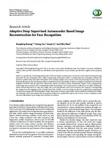
Figure 2. Autoencoder network architecture. The left is encoder network and the right is decoder network.
Gaussian random variable. The other is feature perceptual loss. Instead of directly comparing the input image and the generated image in the pixel space, we feed both of them to a pre-trained deep CNN Φ respectively and then measure the difference between hidden layer representations, i.e., Lrec = L1 + L2 + ... + Ll , where Ll represents the feature loss at the lth hidden layer. Thus, we use the highlevel feature loss to better measure the perceptual and semantic differences between the two images, this is because the pretrained network on image classification has already incorporated perceptual and semantic information we desired for. During the training, the pretrained loss network is fixed and just for high-level feature extraction, and the KL divergence loss Lkl is used to update the encoder network while the feature perceptual loss Lrec is responsible for updating parameters of both the encoder and decoder.
3.1. Variational Autoencoder Network Architecture Both encoder and decoder network are based on deep CNN like AlexNet [13] and VGGNet [29]. We construct 4 convolutional layers in the encoder network with 4 x 4 kernels, and the stride is fixed to be 2 to achieve spatial downsampling instead of using deterministic spatial functions such as maxpooling. Each convolutional layer is followed by a batch normalization layer and a LeakyReLU activation layer. Then two fully-connected output layers (for mean and variance) are added to encoder, and will be used to compute the KL divergence loss and sample latent variable z (see [12] for details). For decoder, we use 4 convolutional layers with 3 x 3 kernels and set stride to be 1, and replace standard zero-padding with replication padding, i.e., feature map of an input is padded with the replication of the input boundary. For upsampling we use nearest neighbor method by a scale of 2 instead of fractional-strided convolutions used by other works [20, 24]. We also use batch normalization to help stabilize training and use LeakyReLU as
the activation function. The details of autoencoder architecture is shown in Figure 2.
3.2. Feature Perceptual Loss Feature perceptual loss of two images is defined as the difference between the hidden features in a pretrained deep convolutional neural network Φ. Similar to [4], we use VGGNet [29] as the loss network in our experiment, which is trained for classification problem on ImageNet dataset. The core idea of feature perceptual loss is to seek the consistency between the hidden representations of two images. As the hidden representations can capture important perceptual quality features such as spatial correlation, smaller difference of hidden representations indicates consistency of spatial correlations between the input and the output, as a result, we can get a better visual quality of the output image. Specifically, let Φ(x)l represent the representation of the lth hidden layer when input image x is fed to network Φ. Mathematically Φ(x)l is a 3D volume block array of the shape [C l x W l x H l ], where C l is the number of filters, W l and H l represent the width and height of each feature map for the lth layer. The feature perceptual loss for one layer (Llrec ) between two images x and x ¯ can be simply defined by squared euclidean distance. Actually it is quite like pixel-by-pixel loss for images except that the color channel is not 3 anymore. l
Llrec =
l
l
C X W X H X 1 (Φ(x)lc,w,h − Φ(¯ x)lc,w,h )2 2C l W l H l c=1 w=1 h=1
(4)
The final reconstruction loss is defined as the total loss by combining different layers of VGG Network, i.e., Lrec = P l L . Additionally we adopt the KL divergence loss Lkl l rec [12] to regularize the encoder network to control the distribution of the latent variable z. To train VAE, we jointly minimize the KL divergence loss Lkl and the feature perceptual loss Llrec for different layers, i.e.,
Ltotal = αLkl + β
l X (Llrec )
(5)
PVAE
i
where α and β are weighting parameters for KL Divergence and image reconstruction. It is quite similar to style transfer [4] if we treat KL Divergence as style reconstruction.
4. Experiments In this paper, we perform experiments on face images to test our method. Specifically we evaluate the image generation performance and compared with other generative models. Furthermore, we also investigate the latent space and study the semantic relationship between different latent representations and apply them to facial attribute prediction.
4.1. Training Details Our model is trained on CelebFaces Attributes (CelebA) Dataset [19]. CelebA is a large-scale face attribute dataset with 202,599 face images, 5 landmark locations, and 40 binary attributes annotations per image. We build the training dataset by cropping and scaling the aligned images to 64 x 64 pixels like [16, 24]. We train our model with a batch size of 64 for 5 epochs over the training dataset and use Adam method for optimization [10] with initial learning rate of 0.0005, which is decreased by a factor of 0.5 for the following epochs. The 19-layer VGGNet [29] is chosen as loss network Φ to construct feature perceptual loss for image reconstruction. We experiment with different layer combinations to construct feature perceptual loss and train two models, i.e., VAE-123 and VAE-345, by using layers relu1 1, relu2 1, relu3 1 and relu3 1, relu4 1, relu5 1 respectively. In addition, the dimension of latent vector z is set to be 100, like DCGAN [24], and the loss weighting parameters α and β are 1 and 0.5 respectively. Our implementation is built on deep learning framework Torch [2]. In this paper, we also train additional two generative models for comparison. One is the plain Variational Autoencoder (PVAE), which has the same architecture as our proposed model, but trained with pixel-by-pixel loss in the image space. The other is Deep Convolutional Generative Adversarial Networks (DCGAN) consisting of a generator and a discriminator network [24], which has shown the ability to generate high quality images from noise vectors. DCGAN is trained with open source code [24] in Torch.
4.2. Qualitative Results for Image Generation The comparison is divided into two parts: arbitrary face images generated by the decoder based on latent vectors z drawn from N (0, 1), and face image reconstruction.
DCGAN
VAE-123
VAE-345
Figure 3. Generated fake face images from 100-dimension latent vector z ∼ N (0, 1) from different models. The first part is generated from the decoder network of plain variational autoencoder (PVAE) trained with pixel-based loss [12], the second part is generated from generator network of DCGAN [24], and the last two parts are the results of VAE-123 and VAE-345 trained with feature perceptual loss based on layers relu1 1, relu2 1, relu3 1, and relu3 1, relu4 1, relu5 1 respectively.
Input PVAE VAE-123 VAE-345
Input PVAE VAE-123 VAE-345
Figure 4. Image reconstruction from different models. The first row is input image, the second row is generated from decoder network of plain variational autoencoder (PVAE) trained with pixelbased loss [12], and the last two rows are the results of VAE-123 and VAE-345 trained with feature perceptual loss based on layers relu1 1, relu2 1, relu3 1, and relu3 1, relu4 1, relu5 1 respectively.
In the first part, random face images (shown in Figure 3) are generated by feeding latent vector z drawn from N (0, 1) to the decoder network in our models and the generator network in DCGAN respectively. We can see that the generated face images by plain VAE tend to be very blurry, even though the overall spatial face structure can be preserved. It is very hard for plain VAE to generate clear fa-
cial parts such as eyes and noses, this is because it tries to minimize the pixel-by-pixel loss between two images. The pixel-based loss does not contain the perceptual and spatial correlation information. DCGAN can generate clean and sharp face images containing clearer facial features, however it has the facial distortion problem and sometimes generates weird faces. Our method based on feature perceptual loss can achieve better results. VAE-123 can generate faces of different genders, ages with clear noses, eyes and teeth, which are better than VAE-345. However, VAE-345 is better at generating hair with different textures. We also compare the reconstruction results (shown in Figure 4) between plain VAE and our two models, and DCGAN is not compared because of no input image in their model. We can get similar conclusion as above. In addition, VAE-123 is better at keeping the original color of input images and generating clearer eyes and teeth. The VAE-345 can generate face images with more realistic hair, but the color could be different from the original in the input images. VAE-345 is trained with higher hidden layers of VGGNet and captures spatial correlation on a coarser scale than VAE-123, hence the images generated by VAE-345 are more blurry than those of VAE-123. Additionally as textures such as hair reflects larger area correlations, this may explain why VAE-345 generates better textures than VAE123. The other way around, local patterns like eyes and noses reflect smaller area correlations, thus VAE-123 can generate clearer eyes and noses than VAE-345.
4.3. The Learned Latent Space In order to get a better understanding of what our model has learned, we investigate the property of the z representation in the latent space, and the relationship between different learned latent vectors. The following experiments are based on our trained VAE-123 model. 4.3.1
Linear Interpolation of Latent Space
As shown in Figure 5, we investigate the linear interpolation between the generated images from two latent vectors denoted as zlef t and zright . The interpolation is defined by linear transformation z = (1 − α)zlef t + αzright , where α = 0, 0.1, . . . , 1, and then z is fed to the decoder network to generate new face images. Here we show three examples for latent vector z encoded from input images and one example for z randomly drawn from N (0, 1). From the first row in Figure 5, we can see the smooth transitions between vector(”Woman without smiling and short hair”) and vector(”Woman with smiling and long hair”). Little by little the hair becomes longer, the distance between lips becomes larger and teeth is shown in the end as smiling, and pose turns from looking slightly right to looking front.
α=0
α=1
z~ !(0, 1)
z~ !(0, 1)
Figure 5. Linear interpolation for latent vector. Each row is the interpolation from left latent vector zlef t to right latent vector zright . e.g. (1 − α)zlef t + αzright . The first row is the transition from a non-smiling woman to a smiling woman, the second row is the transition from a man without eyeglass to a man with eyeglass, the third row is the transition from a man to a woman, and the last row is the transition between two fake faces decoded from z ∼ N (0, 1). α=0
α=1 add smiling vector subtract smiling vector add sunglass vector add sunglass vector subtract sunglass vector
Figure 6. Vector arithmetic for visual attributes. Each row is the generated faces from latent vector zlef t by adding or subtracting an attribute-specific vector, i.e., zlef t + α zsmiling , where α = 0, 0.1, . . . , 1. The first row is the transition by adding a smiling vector with a linear factor α from left to right, the second row is the transition by subtracting a smiling vector, the third and fourth row are the results by adding a eyeglass vector to the latent representation for a man and women, and the last row shows results by subtracting an eyeglass vector.
Additionally we provide examples of transitions between vector(”Man without eyeglass”) and vector(”Man with eyeglass”), and vector(”Man”) and vector(”Woman”). 4.3.2
Facial Attribute Manipulation
The experiments above demonstrate interesting smooth transitional property between two learned latent vectors. In this part, instead of manipulating the overall face images, we seek to find a way to control a specific attribute of face images. In previous works, [22] shows that vector(”King”) - vector(”Man”) + vector(”Woman”) generates a vector whose nearest neighbor is the vector(”Queen”) when evaluating learned representation of words. [24] demonstrates that visual concepts such as face pose and gender could be manipulated by simple vector arithmetic. In this paper, we
ec kl a ou ce ng Y
N
ttr ac Ba tive ld Ba ng s Bl on d_ Ey Ha eg ir la s G ra ses y_ M Ha ak ir eu M p al e Pa le _S Sm kin ili n H g at
A Attractive
1
Bald
0.8
Bangs
0.6
Blond_Hair
0.4
Eyeglasses Gray_Hair Makeup Male
0.2 0 -0.2
Pale_Skin Smiling Hat Necklace
-0.4 -0.6 -0.8
Young
is the same as calculating eyeglass-specific vector above). We then calculate the correlation matrix (Pearson’s correlation) of the 13 attribute-specific vectors, and visualize it as shown in Figure 7. The results are consistent with human interpretation. We can see that Attractive has a strong positive correlation with M akeup, and a negative correlation with M ale and Gray Hair. It makes sense that female is generally considered more attractive than male and uses more makeup. Similarly, Bald has a positive correlation with Gray Hair and Eyeglasses, and a negative correlation with Y oung. Additionally, Smiling seems to have no correlation with most of other attributes and only has a weak negative correlation with P ale Skin. It could be explained that Smiling is a very common human facial expression and it could have a good match with many other attributes.
-1
4.3.4 Figure 7. Diagram for the correlation between selected facial attribute-specific vectors. The blue indicates positive correlation, while red represents negative correlation, and the color shade and size of the circle represent the strength of the correlation.
investigate two facial attributes wearing eyeglass and smiling. We randomly choose 1,000 face images with eyeglass and 1,000 without eyeglass respectively from the CelebA dataset [19]. The two types of images are fed to our encoder network to compute the latent vectors, and the mean latent vectors are calculated for each type respectively, denoted as zpos eyeglass and zneg eyeglass . We then define the difference zpos eyeglass − zneg eyeglass as eyeglass-specific latent vector zeyeglass . In the same way, we calculate the smiling-specific latent vector zsmiling . Then we apply the two attribute-specific vectors to different latent vectors z by simple vector arithmetic like z + α zsmiling . As shown in Figure 6, by adding a smiling vector to the latent vector of a non-smiling man, we can observe the smooth transitions from non-smiling face to smiling face (the first row). Furthermore, the smiling appearance becomes more obvious when the factor α is bigger, while other facial attributes are able to remain unchanged. The other way around, when the latent vector of smiling woman is subtracted by the smiling vector, the smiling face can be translated to not smiling by only changing the shape of mouth (the second row in Figure 6). Moreover, we could add or wipe out an eyeglass by playing with the calculated eyeglass vector. 4.3.3
Correlation Between Attribute-specific Vectors
Considering the conceptual relationship between different facial attributes in natural images, for instance, bald and gray hair are often related to old people. We selected 13 of 40 attributes from CelebA dataset and calculate their attribute-specific latent vectors respectively (the calculation
Visualization of Latent Vectors
Considering that the latent vectors are nothing but the encoding representation of the natural face images, we think that it may be interesting to visualize the natural face images based on the similarity of their latent representations. Specifically we randomly choose 1600 face images from CelebA dataset and extract the corresponding 100dimensional latent vectors, which are then reduced to 2dimensional embedding by t-SNE algorithm [21]. t-SNE can arrange images that have similar high-dimensional vectors (L2 distance) to be nearby each other in the embedding space. The visualization of 40 x 40 images is shown in Figure 8. We can see that images with similar background (black or white) tend to be clustered as a group, and females with smiling are clustered together (green rectangle in Figure 8). Furthermore, the face pose information can be also captured even no pose annotations in the dataset. The face images in the upper left (blue rectangle) are those looking to the right and samples in the bottom left (red rectangle) are those looking to the left, while in other area the faces look to the front. 4.3.5
Facial Attribute Prediction
We further evaluate our model by applying the latent vector to facial attribute prediction, which is a very challenging problem. Similar to [19], 20,000 images from CelebA dataset are selected for testing and the rest for training. Instead of using a face detector, we use ground truth landmark points to crop out the face parts of the original images like PANDA-l [34], and the cropped face images are fed to our encoder network to extract the latent vectors for both VAE-123 and VAE-345, which are then used to train standard Linear SVM [23] classifiers with the corresponding 40 binary attributes annotations per image provide by CelebA. As a result, we train 40 binary classifiers for each attribute in CelebA dataset respectively. As a baseline, we
Looking Right
Looking Left
Figure 8. Visualization of 40 x 40 face images based on latent vectors by t-SNE algorithm [21].
also train different Linear SVM classifiers for each attribute with 4096-dimensional deep features extracted from the last fully connected layer of pretrained VGGNet [29]. We then compare our method with other state-of-theart methods. The average of prediction accuracies of FaceTracer [14], PANDA-w [34], PANDA-l [34], and LNets+ANet [19] are 81.13, 79.85, 85.43 and 87.30 percent respectively. The results of our method with latent vectors of VAE-123 and VAE-345 are 86.95 and 88.73 respectively, whilst that of VGG last layer features (VGG-FC) is 79.85. From Table 1, we can see that our method VAE-
345 outperforms other methods. In addition, we notice that all the methods can achieve a good performance to predict Bald, Eyeglasses and W earing Hat while it is difficult for them to correctly predict attributes like Big Lips and Oval F ace. It might be explained that attributes like wearing hat and eyeglasses are much more obvious in face images, than attributes like big lips and Oval face, and the extracted features are not able to capture such subtle differences. Future work is needed to find a way to extract better features which can also capture these tiny variations of facial attributes.
H. Cheekbones
Male
85 84 90 90 85 89 79
84 80 86 87 81 85 64
91 93 97 98 90 95 84
Method
Average
Heavy Makeup
90 88 94 97 96 97 94
Young
Gray Hair
93 86 93 95 94 95 93
Wear. Necktie
Goatee
98 94 98 99 96 99 95
Wear. Necklace
Eyeglasses
88 85 88 92 95 96 93
Wear. Lipstick
Double Chin
86 82 86 91 94 94 93
Wear. Hat
Chubby
80 76 86 90 87 88 81
Wear. Earrings
Bushy Eyebrows
60 69 77 80 80 80 67
Wavy Hair
Brown Hair
81 77 86 84 95 95 94
Straight Hair
Blurry
80 81 93 95 92 93 88
Smiling
Blond Hair
70 74 85 88 83 85 78
Sideburns
Black Hair
74 70 75 78 79 81 77
Rosy Cheeks
Big Nose
64 61 67 68 76 77 51
Reced. Hairline
Big Lips
88 89 92 95 91 95 81
Pointy Nose
Bangs
89 92 96 98 98 98 97
Pale Skin
Bald
76 71 79 79 81 82 73
Oval Face
Bags Un. Eyes
78 77 81 81 75 78 68
No Beard
Attractive
76 73 78 79 77 80 71
Narrow Eyes
Arch. Eyebrows
85 82 88 91 89 89 83
Mustache
5 Shadow
FaceTracer PANDA-w PANDA-l LNets+ANet VAE-123 VAE-345 VGG-FC
Mouth S. O.
Method
FaceTracer PANDA-w PANDA-l LNets+ANet VAE-123 VAE-345 VGG-FC
87 82 93 92 80 88 60
91 83 93 95 96 96 93
82 79 84 81 89 89 87
90 87 93 95 88 91 84
64 62 65 66 73 74 66
83 84 91 91 96 96 96
68 65 71 72 73 74 58
76 82 85 89 92 92 86
84 81 87 90 94 94 93
94 90 93 96 95 96 85
89 89 92 92 87 91 65
63 67 69 73 79 80 68
73 76 77 80 74 79 70
73 72 78 82 82 84 49
89 91 96 99 96 98 98
89 88 93 93 88 91 82
68 67 67 71 88 88 87
86 88 91 93 93 93 89
80 77 84 87 81 84 74
81.13 79.85 85.43 87.30 86.95 88.73 79.85
Table 1. Performance comparison of 40 facial attributes prediction. The accuracies of FaceTracer [14], PANDA-w [34], PANDA-l [34], and LNets+ANet [19] are collected from [19]. PANDA-l, VAE-123, VAE-345 and VGG-FC use the truth landmarks to get the face part.
4.4. Discussion For AVE models, one essential part is to define a reconstruction loss to measure the similarity between the input and the generated image. The plain VAE adopts the pixelby-pixel distance, which is problematic and the generated images tend to be very blurry. Inspired by the recent works like style transfer and texture synthesis [4, 8, 30], feature perceptual loss based on pretrained deep CNNs are used to improve the performance of VAE to generate high quality images in our work. One explanation is that the hidden representation in a pretrained deep CNN could capture essential visual quality factors such as spatial correlation information of a given image. Another benefit of using deep CNNs is that we can combine different level of hidden representations, which can provide more constraints for the reconstruction. However, the feature perceptual loss is not perfect, trying to construct better reconstruction loss to measure the similarity of the output images and groundtruth images is essential for further work. One possibility is to combine feature perceptual loss with generative adversarial networks(GAN). Another interesting part of VAE is the linear structure in the learned latent space. Different images generated by the decoder can be smoothly transformed to each other by simple linear combination of their latent vectors. Additionally attribute-specific latent vectors could be also calculated by encoding the annotated images and used to manipulate the
related attribute of a given image while keeping other attributes unchanged. Furthermore, the correlation between attribute-specific vectors shows consistency with high level understanding. Our experiments shows that the learned latent space of VAE can learn powerful representation of conceptual and semantic information of face images, and it could be used for other applications like face attribute prediction.
5. Conclusion In this paper, we propose to train a deep feature consistent variational autoencoder by feature perceptual loss based on pretrained deep CNNs to measure the similarity of the input and generated images. We apply our model on face image generation and achieve comparable and even better performance when compared to different generative models. In addition, we explore the learned latent representation in our model and demonstrate that it has powerful capability of capturing the conceptual and semantic information of natural (face) images. We also achieve state-ofthe-art performance in facial attribute prediction based on the learned latent representation.
References [1] A. Babenko, A. Slesarev, A. Chigorin, and V. Lempitsky. Neural codes for image retrieval. In Computer Vision–ECCV 2014, pages 584–599. Springer, 2014.
[2] R. Collobert, K. Kavukcuoglu, and C. Farabet. Torch7: A matlab-like environment for machine learning. In BigLearn, NIPS Workshop, number EPFL-CONF-192376, 2011. [3] L. Gatys, A. S. Ecker, and M. Bethge. Texture synthesis using convolutional neural networks. In Advances in Neural Information Processing Systems, pages 262–270, 2015. [4] L. A. Gatys, A. S. Ecker, and M. Bethge. A neural algorithm of artistic style. arXiv preprint arXiv:1508.06576, 2015. [5] R. Girshick, J. Donahue, T. Darrell, and J. Malik. Rich feature hierarchies for accurate object detection and semantic segmentation. In Proceedings of the IEEE conference on computer vision and pattern recognition, pages 580–587, 2014. [6] I. Goodfellow, J. Pouget-Abadie, M. Mirza, B. Xu, D. Warde-Farley, S. Ozair, A. Courville, and Y. Bengio. Generative adversarial nets. In Advances in Neural Information Processing Systems, pages 2672–2680, 2014. [7] K. Gregor, I. Danihelka, A. Graves, D. J. Rezende, and D. Wierstra. Draw: A recurrent neural network for image generation. arXiv preprint arXiv:1502.04623, 2015. [8] J. Johnson, A. Alahi, and L. Fei-Fei. Perceptual losses for real-time style transfer and super-resolution. arXiv preprint arXiv:1603.08155, 2016. [9] A. Karpathy and L. Fei-Fei. Deep visual-semantic alignments for generating image descriptions. In Proceedings of the IEEE Conference on Computer Vision and Pattern Recognition, pages 3128–3137, 2015. [10] D. Kingma and J. Ba. Adam: A method for stochastic optimization. arXiv preprint arXiv:1412.6980, 2014. [11] D. P. Kingma, S. Mohamed, D. J. Rezende, and M. Welling. Semi-supervised learning with deep generative models. In Advances in Neural Information Processing Systems, pages 3581–3589, 2014. [12] D. P. Kingma and M. Welling. Auto-encoding variational bayes. arXiv preprint arXiv:1312.6114, 2013. [13] A. Krizhevsky, I. Sutskever, and G. E. Hinton. Imagenet classification with deep convolutional neural networks. In Advances in neural information processing systems, pages 1097–1105, 2012. [14] N. Kumar, P. Belhumeur, and S. Nayar. Facetracer: A search engine for large collections of images with faces. In European conference on computer vision, pages 340–353. Springer, 2008. [15] A. Lamb, V. Dumoulin, and A. Courville. Discriminative regularization for generative models. arXiv preprint arXiv:1602.03220, 2016. [16] A. B. L. Larsen, S. K. Sønderby, and O. Winther. Autoencoding beyond pixels using a learned similarity metric. arXiv preprint arXiv:1512.09300, 2015. [17] J. C. Leachtenauer, W. Malila, J. Irvine, L. Colburn, and N. Salvaggio. General image-quality equation: Giqe. Applied Optics, 36(32):8322–8328, 1997. [18] C. Li and M. Wand. Combining markov random fields and convolutional neural networks for image synthesis. arXiv preprint arXiv:1601.04589, 2016. [19] Z. Liu, P. Luo, X. Wang, and X. Tang. Deep learning face attributes in the wild. In Proceedings of the IEEE International Conference on Computer Vision, pages 3730–3738, 2015.
[20] J. Long, E. Shelhamer, and T. Darrell. Fully convolutional networks for semantic segmentation. In Proceedings of the IEEE Conference on Computer Vision and Pattern Recognition, pages 3431–3440, 2015. [21] L. v. d. Maaten and G. Hinton. Visualizing data using t-sne. Journal of Machine Learning Research, 9(Nov):2579–2605, 2008. [22] T. Mikolov and J. Dean. Distributed representations of words and phrases and their compositionality. Advances in neural information processing systems, 2013. [23] F. Pedregosa, G. Varoquaux, A. Gramfort, V. Michel, B. Thirion, O. Grisel, M. Blondel, P. Prettenhofer, R. Weiss, V. Dubourg, J. Vanderplas, A. Passos, D. Cournapeau, M. Brucher, M. Perrot, and E. Duchesnay. Scikit-learn: Machine learning in Python. Journal of Machine Learning Research, 12:2825–2830, 2011. [24] A. Radford, L. Metz, and S. Chintala. Unsupervised representation learning with deep convolutional generative adversarial networks. arXiv preprint arXiv:1511.06434, 2015. [25] D. J. Rezende, S. Mohamed, and D. Wierstra. Stochastic backpropagation and approximate inference in deep generative models. In Proceedings of the 31st International Conference on Machine Learning (ICML-14), pages 1278–1286, 2014. [26] K. Ridgeway, J. Snell, B. Roads, R. Zemel, and M. Mozer. Learning to generate images with perceptual similarity metrics. arXiv preprint arXiv:1511.06409, 2015. [27] O. Russakovsky, J. Deng, H. Su, J. Krause, S. Satheesh, S. Ma, Z. Huang, A. Karpathy, A. Khosla, M. Bernstein, A. C. Berg, and L. Fei-Fei. ImageNet Large Scale Visual Recognition Challenge. International Journal of Computer Vision (IJCV), 115(3):211–252, 2015. [28] K. Simonyan, A. Vedaldi, and A. Zisserman. Deep inside convolutional networks: Visualising image classification models and saliency maps. arXiv preprint arXiv:1312.6034, 2013. [29] K. Simonyan and A. Zisserman. Very deep convolutional networks for large-scale image recognition. arXiv preprint arXiv:1409.1556, 2014. [30] D. Ulyanov, V. Lebedev, A. Vedaldi, and V. Lempitsky. Texture networks: Feed-forward synthesis of textures and stylized images. arXiv preprint arXiv:1603.03417, 2016. [31] Z. Wang and A. C. Bovik. A universal image quality index. IEEE signal processing letters, 9(3):81–84, 2002. [32] X. Yan, J. Yang, K. Sohn, and H. Lee. Attribute2image: Conditional image generation from visual attributes. arXiv preprint arXiv:1512.00570, 2015. [33] J. Yosinski, J. Clune, A. Nguyen, T. Fuchs, and H. Lipson. Understanding neural networks through deep visualization. arXiv preprint arXiv:1506.06579, 2015. [34] N. Zhang, M. Paluri, M. Ranzato, T. Darrell, and L. Bourdev. Panda: Pose aligned networks for deep attribute modeling. In Proceedings of the IEEE Conference on Computer Vision and Pattern Recognition, pages 1637–1644, 2014.