Adaptive Deep Supervised Autoencoder Based Image Reconstruction

Hindawi Publishing Corporation Mathematical Problems in Engineering Volume 2016, Article ID 6795352, 14 pages http://dx.doi.org/10.1155/2016/6795352

Research Article Adaptive Deep Supervised Autoencoder Based Image Reconstruction for Face Recognition Rongbing Huang,1,2 Chang Liu,1 Guoqi Li,3 and Jiliu Zhou2 1

Key Laboratory of Pattern Recognition and Intelligent Information Processing, Institutions of Higher Education of Sichuan Province, Chengdu University, Chengdu, Sichuan 610106, China 2 School of Computer and Software, Sichuan University, Chengdu, Sichuan 610065, China 3 School of Reliability and System Engineering, Beihang University, Beijing 100191, China Correspondence should be addressed to Rongbing Huang; [email protected] Received 3 June 2016; Revised 30 July 2016; Accepted 28 September 2016 Academic Editor: Simone Bianco Copyright © 2016 Rongbing Huang et al. This is an open access article distributed under the Creative Commons Attribution License, which permits unrestricted use, distribution, and reproduction in any medium, provided the original work is properly cited. Based on a special type of denoising autoencoder (DAE) and image reconstruction, we present a novel supervised deep learning framework for face recognition (FR). Unlike existing deep autoencoder which is unsupervised face recognition method, the proposed method takes class label information from training samples into account in the deep learning procedure and can automatically discover the underlying nonlinear manifold structures. Specifically, we define an Adaptive Deep Supervised Network Template (ADSNT) with the supervised autoencoder which is trained to extract characteristic features from corrupted/clean facial images and reconstruct the corresponding similar facial images. The reconstruction is realized by a so-called “bottleneck” neural network that learns to map face images into a low-dimensional vector and reconstruct the respective corresponding face images from the mapping vectors. Having trained the ADSNT, a new face image can then be recognized by comparing its reconstruction image with individual gallery images, respectively. Extensive experiments on three databases including AR, PubFig, and Extended Yale B demonstrate that the proposed method can significantly improve the accuracy of face recognition under enormous illumination, pose change, and a fraction of occlusion.

1. Introduction Over the last couple of decades, face recognition has gained a great deal of attention in the academic and industrial communities on account of its challenging essence and its widespread applications. The study of face recognition has a great theoretical value, which involves image processing, artificial intelligence, machine learning, computer vision, and so on, and it also has a high correlation with other biometrics like fingerprints, speech recognition, and iris scans. In the field of pattern recognition, as a classic problem, face recognition mainly covers two issues, feature exaction and classifier design. Currently, most existing works are focusing on these two aspects to promote the performance of face recognition system. In most real-world applications, it is actually a multiclass classification issue for face recognition. There are many classification methods proposed by researchers. Among them,

nearest neighbor classifier (NNC) and its variants like nearest subspace [1] are the most popular methods in pattern classification [2]. In [3], the problem of face recognition was transformed to a binary classification problem through constructing intra- and interfacial image spaces. The intraspace stands for the difference of the same person and the interspace denotes the difference of different people. Then, many binary classifiers such as Support Vector Machine (SVM) [4], Bayesian, and Adaboost [5] can be used. Besides the classifier design, the other important issue is feature representation. In the real word, face images are usually influenced by variances such as illuminations, posture, occlusions, and expressions. Additionally, there is fact that the difference from the same person would be much larger than that from different people. Therefore, it is crucial to get efficient and discriminant features making the intraspace compact and expanding the margin among different people. Until now, various feature extraction methods

2

Mathematical Problems in Engineering

1024 Decoder

x̂

···

2000

1256

ℎ

···

250

̂ ‖x − x‖ x̃

2

1256

···

2000

x

···

1024

(a)

Encoder

(b)

Figure 1: Network architectures. (a) DAE and (b) SDAE.

have been explored, including classical subspace-based dimension reduction approaches like principal component analysis (PCA), fisher linear discriminant analysis (FLDA), independent component analysis (ICA), and so on [6]. In addition, there are some local appearance features extraction methods like Gabor wavelet transform, local binary patterns (LBP), and their variants [7] which are stable to local facial variations such as expressions, occlusions, and poses. Currently, deep learning including deep neural network has shown its great success on image expression [8, 9], and their basic idea is to train a nonlinear feature extractor in each layer [10, 11]. After greedy layer-wise training of a deep network architecture, the output of the network is applied as image feature for latter classification task. Among deep network architectures, as a representative building block, denoising autoencoder (DAE) [12] learns features that is robust to noise by a nonlinear deterministic mapping. Image features derived from DAE have demonstrated good performance in many aspects such as object detection and digit recognition. Inspired by the great success of DAE based deep network architecture, a supervised autoencoder (SAE) [9] was also proposed to build the block, which firstly treated the facial images in some variants like illuminations, expressions, and poses as corrupted images by noises. A face image without the variant through an SAE can be recovered; meanwhile, robust features for image representation are also extracted. Taking as an example the great success of DAE and SAE based deep learning and inspired by the face recognition under complex environment, in this article, we present a novel deep learning method based on SAE for face recognition. Unlike existing deep stacked autoencoder (AE) which is an unsupervised feature learning approach, our proposed method takes full advantage of the class label information of training samples in the deep learning procedure and tries to discover the underlying nonlinear manifold structures in the data.

The rest of this paper is organized as follows. In Section 2, we give a brief review of DAE and the state-of-the-art face recognition based on deep learning. In Section 3, we focus on the proposed face recognition approach. The experimental results conducted on three public databases are given in Section 4. Finally, we draw a conclusion in Section 5.

2. Related Work In this section, we briefly review work related to DAE and deep learning based face recognition system. 2.1. Work Related to DAE. DAE is a one-layer neural network, which is a recent variant of the conventional autoencoder (AE). It learns to try to recover the clean input data sample from its corrupted version. The architecture of DAE is illustrated in Figure 1(a). Let there be a total of 𝑘 training samples and let 𝑥 denote the original input data. In DAE, firstly, let the input data 𝑥 be contaminated with some predefined noise such as Gaussian white noise or Poisson noise to obtain ̃ such that 𝑥 ̃ is input into an encoder ℎ = corrupted version 𝑥 𝑥 + 𝑏𝑓 ). Then an output of the encoder ℎ is used 𝑓(̃ 𝑥) = 𝑢𝑓 (𝑊̃ ̂ = 𝑔(ℎ) = 𝑢𝑔 (𝑊󸀠 ℎ+𝑏𝑔 ). Here 𝑢𝑓 and as an input of a decoder 𝑥 𝑢𝑔 are the predefined activation functions such as sigmoid function, hyperbolic tangent function, or rectifier function [13] of encoder and decoder, respectively. 𝑊 ∈ 𝑅𝑑ℎ ×𝑑𝑥 and 𝑊󸀠 ∈ 𝑅𝑑𝑥 ×𝑑ℎ are the network parameters which denote the weights for the encoder and decoder, respectively. 𝑏𝑓 ∈ 𝑅𝑑ℎ and 𝑏𝑔 ∈ 𝑅𝑑𝑥 refer to the bias terms. 𝑑𝑥 and 𝑑ℎ present dimensionality of the original data and the number of hidden neurons, respectively. On the basis of the above definition, a DAE learns by solving a regularized optimization problem as follows: 𝑘

̂ ‖22 + min ∑ ‖𝑥 − 𝑥 󸀠

𝑊,𝑊 ,𝑏𝑓 ,𝑏𝑔 𝑖=1

𝜆 󵄩 󵄩2 (∑ ‖𝑊‖2𝐹 + ∑ 󵄩󵄩󵄩󵄩𝑊󸀠 󵄩󵄩󵄩󵄩𝐹 ) . 2 𝑗 𝑙

(1)


3 ADSNT

Gallery images Training set

Probe images

Preprocess, for example, histogram equalization

Output: label I of the test image 󵄩󵄩 ̂ 󵄩 󵄩󵄩x(t) − xg 󵄩󵄩󵄩 ∀g ∈ 1, 2, . . . , c I = arg min 󵄩󵄩 g 󵄩 󵄩

Train

𝜃ADSNT

Face dataset

Test image

Preprocess, for example, histogram equalization

Map

Figure 2: Flowchart of the proposed ADSNT image reconstruction for face recognition.

Here ‖ ⋅ ‖22 is the reconstruction error and ‖ ⋅ ‖𝐹 denotes the Frobenius norm and 𝜆 is a parameter that balances the reconstruction loss and weight penalty terms. With reconstructing the clean input data from a corrupted version of it, a DAE can explore more robust features than a conventional AE only simply learning the identity mapping. To further promote learning meaningful features, sparsity constraints [14] are utilized to impose on the hidden neurons when the number of hidden neurons is large, which is defined in the light of the Kullback-Leibler (KL) divergence as 𝑚

𝑚

𝑗

𝑗=1

∑ KL (𝜌 || 𝜌𝑗 ) = ∑ 𝜌 log

𝜌 1−𝜌 + (1 − 𝜌) log ( ) , (2) 𝜌𝑗 1 − 𝜌𝑗

where 𝑚 is the number of neurons in one hidden layer, 𝜌𝑗 is determined by taking the average activation of a hidden unit 𝑗 (over all the training set), and 𝜌 is a sparsity parameter (typically a small value). After finishing 𝑓 and 𝑔 learning, the output from encoder ℎ is input to the next layer. Through training such DAE layerwise, stacked denoising autoencoders (SDAE) are then built. Its structure is illustrated in Figure 1(b). In the real-word application, like face recognition, the faces are usually influenced by all kinds of variances such as expression, illumination, pose, and occlusion. To overcome the effect of variances, Gao et al. [9] proposed supervised autoencoder based on the principle of DAE. They treated the training sample (gallery image) from each person with frontal/uniform illumination, neural expression, and without occlusion as clean data and test faces (probe images) accompanied by variances (expression, illumination, occlusion, etc.) as corrupted data. A mapping capturing the discriminant structure of the facial images from different people is learned, while keeping robust to the variances in these faces. Then robust feature is extracted for image presentation and the performance of face recognition is greatly enhanced. 2.2. Deep Learning Based Face Recognition System. In the early face recognition, there have been various face representation methods including hand-crafted or “shallow” learning ways [6, 7]. In recent years, with the development of big data and computer hardware, feature learning based on deep

structure has been greatly successful in image representation field [8, 12, 15, 16]. By means of deep structure learning, the ability of model representation gets great enhancement and we can learn complicated (nonlinear) information from original data effectively. In [16], deep Fisher network was designed through stacking all the Fisher vectors, which greatly performed over conventional Fisher vector representation. Chen et al. [17] proposed marginalized SDAE to learn the optimal closed-form solution, which reduced the computational complexity and improved the scalability of high-dimensional descriptive features. Taigman et al. [18] presented a face verification system based on Convolutional Neural Networks (CNNs), which also obtained high accuracy of verification on the LFW dataset. Zhu et al. [19] designed a network structure that is composed of facial identity-preserving layer and image reconstruction layer, which can reduce intravariance and achieve discriminant information preservation. In [20], Hayat et al. proposed a deep learning framework based on AE with application to image set classification and face recognition, which obtained the best performance comparing with existing state-of-the-art methods. Gao et al. [9] further proposed an SAE which can be used to build the deep architecture and can extract the facial features that are robust to variants. Sun et al. [21] learned multiple convolutional networks (ConvNets) from predicting 10,000 subjects, which generalized well to face verification issue. Furthermore, they improved the ConvNets by incorporating identification and verification missions and enhanced recognition performance [22]. Cai et al. [23] stacked several sparse independent subspace analyses (sISA) to construct deep network structure to learn identity representation.

3. Proposed Method This section presents our proposed approach whose block diagram is illustrated in Figure 2. Firstly, inspired by stacked DAE and SAE [9], we define Adaptive Deep Supervised Network Template (ADSNT) that can learn an underlying nonlinear manifold structure from the facial images. The basic architecture of ADSNT is illustrated in Figure 3(c) and the corresponding details are depicted in Section 3.1. To make

4

Mathematical Problems in Engineering Similar

···

··· f𝜃1 ··· x

f𝜃1 ··· ̃ x

g3 f3 ··· ··· f2 ··· ̂ f1 x ··· ̃ x Similar

f3 ··· f2 ··· f1 ··· x

Similar

g𝜃󳰀

1

··· ̂ x

Similar (a)

g2 ··· ··· ̂ x

g1

(b)

EC

DC

̂) JH (x, x

x ···

̂ x ··· g𝜃󳰀 1 ··· g𝜃󳰀 2 ··· g𝜃󳰀 3 ··· f𝜃 3 ··· f𝜃 2 ··· f𝜃 1 ···

··· ··· ··· ···

f𝜃 3

f𝜃 2 ··· f𝜃 1 ···

̃ x Corrupted face

x Clean face (c)

Figure 3: Architecture of SSAE and ADSNT. (a) Supervised autoencoder (SAE) which is comprised of clean/“corrupted” datum, one hidden layer, and one reconstruction layer by using the “corrupted datum”; (b) stacked supervised autoencoder (SSAE); (c) architecture of the Adaptive Deep Supervised Network Template (ADSNT).

the deep network perform well, similar to [20], we need to give it initialization weights. Then, the preinitialized ADSNT is trained to reconstruct the invariant faces which are insensitive to illumination, pose, and occlusion. Finally, having trained the ADSNT, we use the nearest neighbor classifier to recognize a new face image by comparing its reconstruction image with individual gallery images, respectively. 3.1. Adaptive Deep Supervised Network Template (ADSNT). As presented in Figure 3(c), our ADSNT is a deep supervised autoencoder (DSAE) that consists of two parts: an encoder (EC) and a decoder (DC). Each of them has three hidden layers and they share the third layer, that is, the central hidden layer. The features learned from the hidden layer and the reconstructed clean face are obtained by using the “corrupted” data to train the SSAE. In the process of pretraining, we learn a stack of SAE, each having only one hidden layer of feature detectors. Then, the learned activation features of one SAE are used as “data” for training the next SAE in the stack. Such training is repeated a number of times until we get the desired number of layers. Although we use the basic SAE structure which is shown in Figure 3(a) [9] to construct the stacked supervised autoencoder (SSAE), Gao et al.’s stacked supervised autoencoder only used two hidden layers and

one reconstruction layer. In this paper, we use three hidden layers to compose the encoder and decoder, respectively, whose structures are shown in Figures 3(b) and 3(c). The encoder part tries best to seek a compact low-dimensional meaningful representation of the clean/“corrupted” data. Following the work [20], the encoder can be formulated as a combination of several layers which are connected with a nonlinear activation function 𝑢𝑓 (⋅). We can use a sigmoid function or a rectified linear unit as nonlinear activation to map the clean/“corrupted” data 𝑥/̃ 𝑥 to a representation ℎ as follows: ℎ = 𝑓 (ℎ2 ) = 𝑢𝑓 (𝑊𝑒(3) ℎ2 + 𝑏𝑒(3) ) , ℎ2 = 𝑓 (ℎ1 ) = 𝑢𝑓 (𝑊𝑒(2) ℎ1 + 𝑏𝑒(2) ) , ℎ1 = 𝑓 (𝑥) = 𝑢𝑓 (𝑊𝑒(1) 𝑥 + 𝑏𝑒(1) ) , ℎ = 𝑓 (ℎ2 ) = 𝑢𝑓 (𝑊𝑒(3) ℎ2 + 𝑏𝑒(3) ) , ℎ2 = 𝑓 (ℎ1 ) = 𝑢𝑓 (𝑊𝑒(2) ℎ1 + 𝑏𝑒(2) ) , ̃ + 𝑏𝑒(1) ) , ℎ1 = 𝑓 (̃ 𝑥) = 𝑢𝑓 (𝑊𝑒(1) 𝑥

(3)


5

where 𝑊𝑒(𝑖) ∈ 𝑅𝑑𝑖−1 ×𝑑𝑖 is a weight matrix of the encoder for the 𝑖th layer with 𝑑𝑖 neurons and 𝑏𝑒(𝑖) ∈ 𝑅𝑑𝑖 is the bias vector. The encoder parameters learning are achieved by jointly training the encoder-decoder structure to reconstruct the “corrupt” data by minimizing a cost function (see Section 3.2). Therefore, the decoder can be defined as a combination of several layers integrating a nonlinear activation function 𝑢𝑔 (⋅) which ̃ from the encoder output ℎ. reconstructs the “corrupt” data 𝑥 ̂ of the decoder is given by The reconstructed output 𝑥 ̂ = 𝑔 (𝑥) = 𝑢𝑔 (𝑊𝑑(3) 𝑥 + 𝑏𝑑(3) ) , 𝑥 𝑥 = 𝑔 (𝑥) = 𝑢𝑔 (𝑊𝑑(2) 𝑥 + 𝑏𝑑(2) ) ,

(4)

𝑥 = 𝑔 (ℎ) = 𝑢𝑔 (𝑊𝑑(1) ℎ + 𝑏𝑑(1) ) .

3.2. Formulation of Image Reconstruction Based on ADSNT. Now, we are ready to depict the reconstruction image based on ADSNT. The details are presented as follows. Given a set of 𝑘 classes training images that include gallery images (called clean data) and probe images (called “corrupted” data), and their corresponding class labels 𝑦𝑐 = [1, 2, . . . , 𝑘], the dataset will be used to train ADSNT for feature learning. Let 𝑥̃𝑖 denote a probe image, and 𝑥𝑖 (𝑖 = 1, 2, . . . , 𝑀) present gallery images corresponding to 𝑥̃𝑖 . It is desirable that 𝑥𝑖 and 𝑥̃𝑖 should be similar. Therefore, following the work [9, 22], we obtain the following formulation:

𝜃ADSNT

1 󵄩 󵄩2 ∑ 󵄩󵄩𝑥 − 𝑥̂𝑖 󵄩󵄩󵄩 𝑀 𝑖 󵄩 𝑖 +

+

𝜆 𝜃𝑊 𝑀

󵄩 󵄩2 𝑥𝑖 )󵄩󵄩󵄩 ∑ 󵄩󵄩󵄩𝑓 (𝑥𝑖 ) − 𝑓 (̃ 𝑖

(5)

3 𝜑 3 󵄩󵄩 (𝑖) 󵄩󵄩2 󵄩 󵄩2 (∑ 󵄩󵄩󵄩𝑊𝑒 󵄩󵄩󵄩𝐹 + ∑ 󵄩󵄩󵄩󵄩𝑊𝑑(𝑖) 󵄩󵄩󵄩󵄩𝐹 ) , 2 𝑗 𝑗

where 𝜃ADSNT = {𝜃𝑊, 𝜃𝑏 } (see Section 3.1) are the parameters of ADSNT which is fine-tuned by learning. In this paper, we 𝑇 only explore the tied weights; that is, 𝑊𝑑(3) = 𝑊𝑒(1) , 𝑊𝑑(2) = 𝑇

𝑇

arg min 𝐽reg 𝜃ADSNT

3

5

𝑖

𝑖

(6)

= 𝐽 + 𝛾 (∑ KL (𝜌𝑥 || 𝜌0 ) + ∑ KL (𝜌𝑥̃ || 𝜌0 )) , where 𝜌𝑥 =

1 1 ∑ ( 𝑓 (𝑥𝑖 ) + 1) , 𝑀 𝑖 2

𝜌𝑥̃ =

1 1 𝑥𝑖 ) + 1) , ∑ (𝑓 (̃ 𝑀 𝑖 2

(7)

KL (𝜌 || 𝜌0 )

So, we can describe the complete ADSNT by its parameter 𝜃ADSNT = {𝜃𝑊, 𝜃𝑏 }, where 𝜃𝑊 = {𝑊𝑒(𝑖) , 𝑊𝑑(𝑖) } and 𝜃𝑏 = {𝑏𝑒(𝑖) , 𝑏𝑑(𝑖) }, 𝑖 = 1, 2, 3.

arg min 𝐽 =

Then, we can further modify cost function and obtain the following objection formulation:

𝑊𝑒(2) , and 𝑊𝑑(1) = 𝑊𝑒(3) (see Figure 3(c)). 𝑥̂𝑖 is the reconstruction image of the corrupted image 𝑥̃𝑖 . Like regularization parameter, 𝜆 𝜃𝑊 balances the similarity of the same person 𝑥𝑖 ) as similarly as possible. 𝑓(⋅) is a to preserve 𝑓(𝑥𝑖 ) and 𝑓(̃ nonlinear activation function. 𝜑 is a parameter that balances weight penalty terms and reconstruction loss. ‖ ⋅ ‖𝐹 presents the Frobenius norm and ∑3𝑗 ‖𝑊𝑒(𝑖) ‖2𝐹 + ∑3𝑗 ‖𝑊𝑑(𝑖) ‖2𝐹 ensures small weight values for all the hidden neurons. Furthermore, following the work [9, 14], we impose a sparsity constraint on the hidden layer to enhance learning meaningful features.

= ∑ (𝜌0 log ( 𝑗

𝜌0 1 − 𝜌0 ) + (1 − 𝜌0 ) log ( )) . 𝜌𝑗 1 − 𝜌𝑗

Here the KL divergence between two distributions, that is, 𝜌0 and 𝜌𝑗 that present 𝜌𝑥 or 𝜌𝑥̃ , is calculated. The sparsity 𝜌0 is usually a constant (taking a small value, according to the work [9, 24], it is set to 0.05 in our experiments), whereas 𝜌𝑥 and 𝜌𝑥̃ are the mapping mean activation values from clean data and corrupted data, respectively. 3.3. Optimization of ADSNT. For obtaining the optimization parameter 𝜃ADSNT = {𝜃𝑊, 𝜃𝑏 }, it is important to initialize weights and select an optimization training algorithm. The training will fail if the initialization weights are inappropriate. This is to say, if we give network too large initialization weights, the ADSNT will be trapped in local minimum. If the initialized weights are too small, the ADSNT will encounter the vanishing gradient problem during backpropagation. Therefore, following the work [20, 24], Gaussian Restricted Boltzmann Machines (GRBMs) are adopted to initialize weight parameters by performing pretraining, which has been already applied widely. For more details, we refer the reader to the original paper [24]. After obtaining the initialized weights, the limited memory Broyden-FletcherGoldfarb-Shanno (L-BFGS) optimization algorithm is utilized to learn the parameters as it has better performance and faster convergence than stochastic gradient descent (SGD) and conjugated gradient (CGD) [25]. Algorithm 1 depicts the optimization procedure of ADSNT. Algorithm 1. (learning adaptive deep supervised network template) Input. Training images Ω: 𝑘 classes, and each class is composed of the face with neutral expression, frontal pose, and normal illumination condition (clean data) and random number of variant faces (corrupted data). Number of network layers 𝐿. Iterative number 𝐼, balancing parameters 𝜆, 𝜑 and 𝛾, and convergence error 𝜀. Output. Weight parameters 𝜃ADSNT = {𝜃𝑊, 𝜃𝑏 }

6

Mathematical Problems in Engineering (1) Preprocess all images, namely, perform histogram equalization (2) 𝑋: Randomly select a small subset for each individual from Ω (3) Initialize: Train GRBMs by using 𝑋 to initialize the 𝜃ADSNT = {𝜃𝑊, 𝜃𝑏 } (4) (Optimization by L-BFGS) For 𝑟 = 1, 2, . . . , 𝑅 do Calculate 𝐽reg using (6) If 𝑟 > 1 and |𝐽𝑟 − 𝐽𝑟−1 | < 𝜀, go to Return

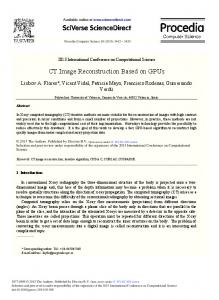
Return. 𝜃𝑊 and 𝜃𝑏 . Since training the ADSNT model aims to reconstruct clean data, namely, gallery images from corrupt data, it might learn an underlying structure from the corrupt data and produce very useful representation. Furthermore, we can learn an overcomplete sparse representation from corrupt data through mapping them into a high-dimensional feature space since the first hidden layer has the number of neurons larger than the dimensionality of original data. The highdimensional model representation is then followed by a socalled “bottleneck”; that is, the data is further mapped to an abstract, compact, and low-dimensional model representation in the subsequent layers of the encoder. Through such a mapping, the redundant information such as illumination, poses, and partial occlusion in the corrupted faces is removed and only the useful information content for us is kept. In addition, we know that if we use AE with only one hidden layer and jointly linear activation functions, the learned weights would be analogous to a PCA subspace [20]. However, AE is an unsupervised algorithm. In our work, we make use of the class label information to train SAE, so if we also use only one hidden layer with a linear activation function, the learned weights by the SAE are thought to be similar to “LDA” subspace. However, in our structure, we apply the nonlinear activation functions and stack several hidden layers together, and then the ADSNT can adapt to very complicated nonlinear manifold structures. Some of reconstructed images based on ADSNT from AR database are shown in Figure 4(b). One can see that ADSNT can remove the illumination. For those face images with partial occlusion, ADSNT can also imitate the clean faces. This results are not surprising because the human being has the capability of inferring the unknown faces from known face images via the experience (for deep network structure, the experience learned derives from generic set) [9]. 3.4. Face Classification Based on ADSNT Image Reconstruction. To better train ADSNT, all images need to be preprocessed. It is a very important step for object recognition including face recognition. The common ways include histogram equalization, geometry normalization, and image smoothing. In this paper, for the sake of simplicity, we only perform histogram equalization on all the facial images to minimize illumination variations. That is, we utilize histogram equalization to normalize the histogram of facial

images and make them more compact. For the details about histogram equalization, one can be referred to see [26]. After the ADSNT is trained completely with a certain number of individuals, we can use it to perform on the unseen face images for recognizing them. Given a test facial image 𝑥(𝑡) which is also preprocessed with histogram equalization in the same way as the training images and presented to the ADSNT network, we reconstruct (𝑡) from ADSNT, which is similar (using (3) and (4)) image 𝑥̂ to clean face. For the sake of simplicity, the nearest neighbor classification based on the Euclidean distance between the reconstruction and all the gallery images identifies the class. The classification formula is defined as 󵄩󵄩󵄩 ̂ 󵄩󵄩 󵄩𝑥(𝑡) − 𝑥𝑔 󵄩󵄩󵄩 , ∀𝑔 ∈ 1, 2, . . . , 𝑐, 𝐼𝑘 (𝑥(𝑡) ) = arg min (8) 󵄩󵄩 󵄩󵄩 𝑔 󵄩 where 𝐼𝑘 (𝑥(𝑡) ) is the resulting identity and 𝑥𝑔 is the clean facial image in the gallery images of individual 𝑔.

4. Experimental Results and Discussion In this section, extensive experiments are conducted to present and compare the performance of different methods with the proposed approach. The experiments are implemented on three widely used face databases, that is, AR [27], Extended Yale B [28], and PubFig [29]. The details of these three databases and performance evaluation of different approaches are presented as follows. 4.1. Dataset Description. The AR database contains over 4000 color face images from 126 people (56 women and 70 men). The images were taken in two sessions (between two weeks) and each session contained 13 pictures from one person. These images contain frontal view faces with different facial expression, illuminations, and occlusions (sun glasses and scarf). Some sample face images from AR are illustrated in Figure 5(a). In our experiments, for each person, we choose the facial images with neutral expression, frontal pose, and normal illumination condition as gallery images and randomly select half the number of images from the rest of the images of each person as probe images. The remaining images compose the testing set. The Extended Yale B database consists of 16128 images of 38 people under 64 illumination conditions and 9 poses. Some sample face images from Extended Yale B are illustrated in Figure 5(b). For each person, we select the faces that have normal light condition and frontal pose as gallery images and randomly choose 6 poses and 16 illumination face images to compose the probe images. The remaining images compose the testing set. The PubFig database is composed of 58,797 images of 200 subjects taken from the internet. The images of the database were taken in completely uncontrolled conditions with noncooperative people. These images have a very large degree of variability in face expression, pose, illumination, and so forth. Some sample images from PubFig are illustrated in Figure 5(c). In our experiments, for each individual, we select the faces with neutral expression, the frontal or


7

(a)

(b)

̃ . (b) Reconstructed Figure 4: Some original images from AR database and the reconstructed ones. (a) Original face images (corrupted faces) 𝑥 ̂. faces 𝑥

near frontal pose, and normal illumination as galleries and randomly choose half the number of images from the rest of the images of each person as probes. The remaining images compose the testing set. 4.2. Experimental Settings. In all the experiments, the facial images from the AR, PubFig, and Extended Yale B databases are automatically detected using OpenCV face detector [30]. After that, we normalize the detected facial images (in orientation and scale) such that two eyes can be aligned at the same location. Then, the face areas are cropped and converted to 256 gray levels images. The size of each cropped image is 26 × 30 pixels. Thus, the dimensionality of the input vector is 780. Figure 6 presents an example from AR database and the corresponding cropped image. Each cropped facial image is further preprocessed with histogram equalization to minimize illumination variations. We train our ADSNT model with 3 hidden layers, where the number of hidden

nodes for these layers is empirically set as [1024 → 500 → 120], because our experiments show that three hidden layers can get a sufficiently good performance (see Section 4.3.3). In order to show the whole experimental process about parameters setting, we initially use the hyperbolic tangent function as the nonlinear activation function and implement ADSNT on AR. We also choose the face images with neutral expression, frontal pose, and normal illumination as galleries and randomly select half the number of images from the rest of the images of each person as probe images. The remaining images compose the testing set. The mean identification rates are recorded. Firstly, we empirically set the parameter 𝜀 = 0.001 and sparsity target 𝜌0 = 0.05 and fix the parameters 𝜆 = 0.5 and 𝜑 = 0.1 in ADSNT to check the effect of 𝛾 on the identification rate. As illustrated in Figure 6(a), where 𝛾 = 0.08, ADSNT recognition method gets the best performance.

8


(a)

(b)

(c)

Figure 5: A fraction of samples from AR, PubFig, and Extended Yale B face databases. (a) AR, (b) Extended Yale B, and (c) PubFig.

Then, according to Figure 6(a), we fix the parameters 𝛾 = 0.08 and 𝜆 = 0.5 in ADSNT to check the influence of 𝜑. As showed in Figure 6(b), when 𝜑 = 0.6, our method achieves the best recognition rate. At last, we fix 𝛾 = 0.08 and 𝜑 = 0.6, and the recognition rates are illustrated in Figure 6(c) with different value of 𝜆. When 𝜆 = 3, the recognition rate is the highest. From the plot in Figure 6, one can observe that the parameters 𝜆, 𝜑, and 𝛾 cannot be too large or too small. If 𝜆 is too large, the ADSNT would be less discriminative of different subjects because it implements too strong similarity preservation entry. But if 𝜆 is too small, it will degrade the recognition performance and the significance of similarity preservation entry. Similarly, 𝛾 can also not be too large, or the hidden neurons will not be activated for a given input

and low recognition rate will be achieved. If 𝛾 is too small, we can get poor performance. For the weight decay 𝜑, if it is too small, the values of weights for all hidden units will change very slightly. On the contrary, the values of weights will change greatly. Using above those experiments, we gain the optimal parameter values used in ADSNT as 𝜆 = 3, 𝜑 = 0.6, and 𝛾 = 0.08 on AR database. The similar experiments also have been performed on Extended Yale B and PubFig databases. We can get the parameters setting as 𝜆 = 2.6, 𝜑 = 0.5, and 𝛾 = 0.06 on Extended Yale B database and 𝜆 = 2.8, 𝜑 = 0.52, and 𝛾 = 0.09 on PubFig database. In the experiments, we use two measures including the mean identification accuracy 𝜇 with standard deviation


9 95 𝜆 = 0.5 𝜑 = 0.1

88

Identification rate (%)

84 80 76

𝛾 = 0.08 𝜆 = 0.5

90 85 80

0.02 0.04 0.08 0 0.1 0.2 0.3 0.4 0.5 0.6 0.7 0.8 0.9 1 2 2.2

0.006

0.0001 0.005 0.001 0.05 0.06 0.07 0.08 0.09 0.1 0.11 0.12 0.13 0.14

75 0.009


92

The parameter 𝛾

The parameter 𝜑

(a)

(b)

𝜑 = 0.6 𝛾 = 0.08


90

85

6.0

5.5

5.0

4.5

4.0

3.5

3.0

2.5

2.0

1.5

1.0

0.5

0.0

80

The parameter 𝜆 (c)

Figure 6: Parameters setting.

](𝜇 ± ]) and the receiving operating characteristic (ROC) curves to validate the effectiveness of our method as well as other methods. 4.3. Experimental Results and Analysis 4.3.1. Comparison with Different Methods. In the following experiments on the three databases, we compare the proposed approach with several recently proposed methods. These compared methods include DAE with 10% random mask noises [12], marginalized DAE (MDAE) [17], Constractive Autoencoders (CAE) [15], Deep Lambertian Networks (DLN) [31], stacked supervised autoencoder (SSAE) [9], ICAReconstruction (RICA) [32], and Template Deep Reconstruction Model (TDRM) [20]. We use the implementation of these algorithms that are provided by the respective authors. For all the compared approaches, we use the default parameters that are recommended in the corresponding papers. The mean identification accuracy with standard deviations of different approaches on three databases is shown in Table 1. The ROC curves of different approaches are illustrated in Figure 7. The results imply that our approach

Table 1: Comparisons of the average identification accuracy and standard deviation (%) of different approaches on different databases. Method DAE [12] MDAE [17] CAE [15] DLN [31] SSAE [9] RICA [32] TDRM [20] Our method

AR 57.56 ± 0.2 67.80 ± 1.3 49.50 ± 2.1 NA 85.21 ± 0.7 76.33 ± 1.7 87.70 ± 0.6 92.32 ± 0.7

Extended Yale B 63.45 ± 1.3 71.56 ± 1.6 55.72 ± 0.8 81.50 ± 1.4 82.22 ± 0.3 70.44 ± 1.3 86.42 ± 1.2 93.66 ± 0.4

PubFig 61.33 ± 1.5 70.55 ± 2.5 68.56 ± 1.6 77.60 ± 1.4 84.04 ± 1.2 72.35 ± 1.5 89.90 ± 0.9 91.26 ± 1.6

significantly outperforms other methods and gets the best mean recognition rates for the same setting of training and testing sets. Compared to those unsupervised deep learning methods such as DAE, MDAE, CAE, DLN, and TDRM, the improvement of our method is over 30% on Extended Yale B and AR databases where there is a little pose variance. On the PubFig database, our approach can also achieve the mean identification rate of 91.26 ± 1.6%

10

Mathematical Problems in Engineering 1.0

1.0

0.8

True positive rate

True positive rate

0.9

0.7 0.6

0.9

0.8

0.5 0.4

0.1

0.2

0.3

0.4 0.5 0.6 0.7 False positive rate

DAE MDAE CAE DLN

0.8

0.9

1.0

SSAE RICA TDRM Our method

0.7

0.0

0.1

0.2

0.3


DAE MDAE CAE SSAE

0.8

0.9

1.0

RICA TDRM Our method

(a)

(b)

1.00 0.95

True positive rate

0.90 0.85 0.80 0.75 0.70 0.65 0.60 0.55 0.50

0.1

0.2

0.3


0.8

0.9

1.0

SSAE RICA TDRM Our method

DAE MDAE CAE DLN

(c)

Figure 7: Comparisons of ROC curves between our method and other methods on different databases. (a) AR, (b) Extended Yale B, and (c) PubFig.

and outperforms all compared methods. The reason is that our method can extract discriminative, robust information to variances (expression, illumination, pose, etc.) in the learned deep networks. Compared with a supervised method like RICA, the proposed method can improve over 16%, 19%, and 23% on AR, PubFig, and Extended Yale B databases, respectively. Our method is a deep learning method, which focuses on the nonlinear classification problem with learning a nonlinear mapping such that more nonlinear, discriminant information may be explored to enhance the identification performance. Compared with SSAE method that is designed for removing the variances such as illumination, pose, and partial occlusion, our method can still be better over 6%

because of using the weight penalty terms, GRBM to initialize weights, and three layers’ similarity preservation term. 4.3.2. Convergence Analysis. In this subsection, we evaluated the convergence of our ADSNT versus a different number of iterations. Figure 8 illustrates the value of the objective function of ADSNT versus a different number of iterations on the AR, PubFig, and Extended Yale B databases. From Figure 8(a), one can observe that ADSNT converges in about 55, 28, and 70 iterations on the three databases, respectively. We also implement the identification accuracy of ADSNT versus a different number of iterations on the AR, PubFig, and Extended Yale B databases. Figure 8(b) plots the mean


11 100

Mean identification rate (%)

Objective function value

4

3

2

1

0

0

30

60 90 Iteration number

120

150

80

60

40

20

AR Extended Yale B PubFig

40 Iteration number

60

80

AR Extended Yale B PubFig (a)

(b)

Figure 8: Convergence analysis. (a) Convergence curves of ADSNT on AR, PubFig, and Extended Yale B. (b) Mean identification rate (%) versus iterations of ADSNT on AR, PubFig, and Extended Yale B.

100

performance of different layer ADSNT. One can observe that three-hidden layer network outperforms 2-layer network, and the result of 3-layer ADSNT network is very nearly equal to those of 4-layer network on AR and Extended Yale B databases. We also observe that the performance of 4-layer network is a bit lower than that of 3-layer network on the PubFig database. In addition, the deeper ADSNT network is, the more complex its computational complexity becomes. Therefore, the 3-layer network depth is a good trade-off between performance and computational complexity.

Identification accuracy (%)

90 80 70 60 50 40 30 20 10 0 AR Layer 1 Layer 2

Extended Yale B

PubFig

Layer 3 Layer 4

Figure 9: The results of ADSNT with different network depth on the different datasets.

4.3.4. Activation Function. Following the work in [9], we also estimate the performance of ADSNT with different activation functions such as sigmoid, hyperbolic tangent, and rectified linear unit (ReLU) [33] which is defined as 𝑓(𝑥) = max(0, 𝑥). When the sigmoid 𝑓(𝑥) = 1/(1 + 𝑒−𝑥 ) is used as activation function, the objective function (see (6)) is rewritten as follows: arg min 𝐽 𝜃ADSNT

identification rate of ADSNT. From Figure 8(b), one can also observe that ADSNT achieves stable performance after about 55, 70, and 28 iterations on AR, PubFig, and Extended Yale B databases, respectively. 4.3.3. The Effect of Network Depth. In this subsection, we conduct experiments on the three face datasets with different hidden layer of our proposed ADSNT network. The proposed method achieves an identification rate of 92.3 ± 0.6%, 93.3 ± 1.2%, and 91.22 ± 0.8% by three-hidden layer ADSNT network, that is, 1024 → 500 → 120, respectively, on AR, Extended Yale B, and PubFig datasets. Figure 9 illustrates the

=

1 󵄩 󵄩2 𝜆 𝜃 󵄩 󵄩2 𝑥𝑖 )󵄩󵄩󵄩 ∑ 󵄩󵄩󵄩𝑥𝑖 − 𝑥̂𝑖 󵄩󵄩󵄩 + 𝑊 ∑ 󵄩󵄩󵄩𝑓 (𝑥𝑖 ) − 𝑓 (̃ 𝑀 𝑖 𝑀 𝑖 +

3 𝜑 3 󵄩󵄩 (𝑖) 󵄩󵄩2 󵄩 󵄩2 (∑ 󵄩󵄩󵄩𝑊𝑒 󵄩󵄩󵄩𝐹 + ∑ 󵄩󵄩󵄩󵄩𝑊𝑑(𝑖) 󵄩󵄩󵄩󵄩𝐹 ) 2 𝑗 𝑗 3

5

𝑖

𝑖

+ 𝛾 (∑ KL (𝜌𝑥 || 𝜌0 ) + ∑ KL (𝜌𝑥̃ || 𝜌0 )) , where 𝜌𝑥 = (1/𝑀) ∑𝑖 𝑓(𝑥𝑖 ), 𝜌𝑥̃ = (1/𝑀) ∑𝑖 𝑓(̃ 𝑥𝑖 ).

(9)

12


Table 2: Comparisons of the ADSNT algorithm with different activation functions on the AR, PubFig, and Extended Yale B databases. Dataset AR Extended Yale B PubFig

Sigmoid 88.66 ± 1.4 90.55 ± 0.6 87.40 ± 1.2

Tanh 92.32 ± 0.7 93.66 ± 0.4 91.26 ± 1.6

ReLU 93.22 ± 1.5 94.54 ± 0.3 92.44 ± 1.1

If ReLU is adopted as activation function, (6) is formulated as arg min 𝐽 𝜃ADSNT

=

1 󵄩 󵄩2 𝜆 𝜃 󵄩 󵄩2 𝑥𝑖 )󵄩󵄩󵄩 ∑ 󵄩󵄩𝑥 − 𝑥̂𝑖 󵄩󵄩󵄩 + 𝑊 ∑ 󵄩󵄩󵄩𝑓 (𝑥𝑖 ) − 𝑓 (̃ 𝑀 𝑖 󵄩 𝑖 𝑀 𝑖 +

3

3

𝜑 󵄩 󵄩2 󵄩 󵄩2 (∑ 󵄩󵄩󵄩󵄩𝑊𝑒(𝑖) 󵄩󵄩󵄩󵄩𝐹 + ∑ 󵄩󵄩󵄩󵄩𝑊𝑑(𝑖) 󵄩󵄩󵄩󵄩𝐹 ) 2 𝑗 𝑗 3

5

𝑖

𝑖

Table 3: (a) Training time (seconds) for different methods. (b) Testing time (seconds) for different methods. The proposed method costs the least amount of testing time comparing with other methods. (a)

Methods DAE [12] MDAE [17] CAE [15] DLN [31] SSAE [9] RICA [32] TDRM [20] Our method

Time 8.61 10.54 7.86 23.43 53.51 13.44 110.2 122.32 (b)

(10)

󵄩 󵄩 󵄩 󵄩 𝑥𝑖 )󵄩󵄩󵄩1 ) . + 𝛾 (∑ 󵄩󵄩󵄩𝑓 (𝑥𝑖 )󵄩󵄩󵄩1 + ∑ 󵄩󵄩󵄩𝑓 (̃ Table 2 shows the performance of the proposed ADSNT based on different activation functions conducted on the three databases. From Table 2, one can see that ReLU achieves the best performance. The key reason is that we use the weight decay term 𝜑 to optimize the objective function. 4.3.5. Timing Consumption Analysis. In this subsection, we use a HP Z620 workstation with Intel Xeon E5-2609, 2.4 GHz CPU, 8 G RAM and conduct a series of experiments on AR database to compare the time consumption of different methods which are tabulated in Table 3. The training time (seconds) is shown in Table 3(a) while the time (seconds) needed to recognize a face from the testing set is shown in Table 3(b). From Table 3, one can see that the proposed method requires comparatively more time for training because of initialization of ADSNT and performing image reconstruction. However, the procedure of training is offline. When we identity an image from testing set, our method requires less time than other methods.

5. Conclusions In this article, we present an adaptive deep supervised autoencoder based image reconstruction method for face recognition. Unlike conventional deep autoencoder based face recognition method, our method considers the class label information from training samples in the deep learning procedure and can automatically discover the underlying nonlinear manifold structures. Specifically, a multilayer supervised adaptive network structure is presented, which is trained to extract characteristic features from corrupted/clean facial images and reconstruct the corresponding similar facial images. The reconstruction is realized by a socalled “bottleneck” neural network that learns to map face

Methods DAE [12] MDAE [17] CAE [15] DLN [31] SSAE [9] RICA [32] TDRM [20] Our method

Time 0.27 0.3 0.26 0.35 0.22 0.19 0.18 0.13

images into a low-dimensional vector and to reconstruct the respective corresponding face images from the mapping vectors. Having trained the ADSNT, a new face image can then be recognized by comparing its reconstruction image with individual gallery images during testing. The proposed method has been evaluated on the widely used AR, PubFig, and Extended Yale B databases and the experimental results have shown its effectiveness. For future work, we are focusing on applying our proposed method to other application fields such as pattern classification based on image set and action recognition based on the video to further demonstrate its validity.

Competing Interests The authors declare that there is no conflict of interests regarding the publication of this paper.

Acknowledgments This paper is partially supported by the research grant for the Natural Science Foundation from Sichuan Provincial Department of Education (Grant no. 13ZB0336) and the National Natural Science Foundation of China (Grant no. 61502059).

References [1] J.-T. Chien and C.-C. Wu, “Discriminant waveletfaces and nearest feature classifiers for face recognition,” IEEE Transactions on


[2]

[3]

[4]

[5] [6]

[7]

[8]

[9]

[10]

[11]

[12]

[13]

[14]

[15]

[16]

[17]

Pattern Analysis and Machine Intelligence, vol. 24, no. 12, pp. 1644–1649, 2002. Z. Lei, M. Pietik¨ainen, and S. Z. Li, “Learning discriminant face descriptor,” IEEE Transactions on Pattern Analysis and Machine Intelligence, vol. 36, no. 2, pp. 289–302, 2014. B. Moghaddam, T. Jebara, and A. Pentland, “Bayesian face recognition,” Pattern Recognition, vol. 33, no. 11, pp. 1771–1782, 2000. N. Cristianini and J. S. Taylor, An Introduction to Support Vector Machines and Other Kernel-based Learning Methods, Cambridge University Press, New York, NY, USA, 2004. R. O. Duda, P. E. Hart, and D. G. Stork, Pattern Classification, John Wiley & Sons, New York, NY, USA, 2nd edition, 2001. W. Zhao, R. Chellappa, P. J. Phillips, and A. Rosenfeld, “Face recognition: a literature survey,” ACM Computing Surveys, vol. 35, no. 4, pp. 399–458, 2003. B. Zhang, S. Shan, X. Chen, and W. Gao, “Histogram of Gabor phase patterns (HGPP): a novel object representation approach for face recognition,” IEEE Transactions on Image Processing, vol. 16, no. 1, pp. 57–68, 2007. A. Krizhevsky, I. Sutskever, and G. E. Hinton, “ImageNet classification with deep convolutional neural networks,” in Neural Information Processing Systems, pp. 1527–1554, 2012. S. Gao, Y. Zhang, K. Jia, J. Lu, and Y. Zhang, “Single sample face recognition via learning deep supervised autoencoders,” IEEE Transactions on Information Forensics and Security, vol. 10, no. 10, pp. 2108–2118, 2015. G. E. Hinton and R. R. Salakhutdinov, “Reducing the dimensionality of data with neural networks,” American Association for the Advancement of Science. Science, vol. 313, no. 5786, pp. 504–507, 2006. Y. Bengio, “Practical recommendations for gradient-based training of deep architecturesm,” in Neural Networks: Tricks of the Trade, pp. 437–478, Springer, Berlin, Germany, 2012. P. Vincent, H. Larochelle, I. Lajoie, Y. Bengio, and P.-A. Manzagol, “Stacked denoising autoencoders: learning useful representations in a deep network with a local denoising criterion,” Journal of Machine Learning Research (JMLR), vol. 11, no. 5, pp. 3371–3408, 2010. V. Nair and G. E. Hinton, “Rectified linear units improve Restricted Boltzmann machines,” in Proceedings of the 27th International Conference on Machine Learning (ICML ’10), pp. 807–814, Haifa, Israel, June 2010. A. Coates, H. Lee, and A. Y. Ng, “An analysis of single-layer networks in unsupervised feature learning,” in Proceedings of the 14th International Conference on Artificial Intelligence and Statistics (AISTATS ’11), pp. 215–223, Sardinia, Italy, 2010. S. Rifai, P. Vincent, X. Muller, X. Glorot, and Y. Bengio, “Contractive auto-encoders: explicit invariance during feature extraction,” in Proceedings of the 28th International Conference on Machine Learning (ICML ’11), pp. 833–840, Bellevue, Wash, USA, July 2011. K. Simonyan, A. Vedaldi, and A. Zisserman, “Deep fisher networks for large-scale image classification,” in Proceedings of the 27th Annual Conference on Neural Information Processing Systems (NIPS ’13), pp. 163–171, Lake Tahoe, Nev, USA, December 2013. M. Chen, Z. Xu, K. Q. Weinberger, and F. Sha, “Marginalized denoising autoencoders for domain adaptation,” in Proceedings of the 29th International Conference on Machine Learning (ICML ’12), pp. 767–774, Edinburgh, UK, July 2012.

13 [18] Y. Taigman, M. Yang, M. Ranzato, and L. Wolf, “DeepFace: closing the gap to human-level performance in face verification,” in Proceedings of the 27th IEEE Conference on Computer Vision and Pattern Recognition (CVPR ’14), pp. 1701–1708, June 2014. [19] Z. Zhu, P. Luo, X. Wang, and X. Tang, “Deep learning identitypreserving face space,” in Proceedings of the 14th IEEE International Conference on Computer Vision (ICCV ’13), pp. 113–120, Sydney, Australia, December 2013. [20] M. Hayat, M. Bennamoun, and S. An, “Deep reconstruction models for image set classification,” IEEE Transactions on Pattern Analysis and Machine Intelligence, vol. 37, no. 4, pp. 713– 727, 2015. [21] Y. Sun, X. Wang, and X. Tang, “Deep learning face representation from predicting 10,000 classes,” in Proceedings of the 27th IEEE Conference on Computer Vision and Pattern Recognition (CVPR ’14), pp. 1891–1898, Columbus, Ohio, USA, June 2014. [22] Y. Sun, X. Wang, and X. Tang, “Deep learning face representation by joint identification-verification,” Tech. Rep., https://arxiv.org/abs/1406.4773. [23] X. Cai, C. Wang, B. Xiao, X. Chen, and J. Zhou, “Deep nonlinear metric learning with independent subspace analysis for face verification,” in Proceedings of the 20th ACM International Conference on Multimedia (MM ’12), pp. 749–752, November 2012. [24] G. E. Hinton, S. Osindero, and Y.-W. Teh, “A fast learning algorithm for deep belief nets,” Neural Computation, vol. 18, no. 7, pp. 1527–1554, 2006. [25] Q. V. Le, J. Ngiam, A. Coates, A. Lahiri, B. Prochnow, and A. Y. Ng, “On optimization methods for deep learning,” in Proceedings of the 28th International Conference on Machine Learning (ICML ’11), pp. 265–272, Bellevue, Wash, USA, July 2011. [26] C. Zhou, X. Wei, Q. Zhang, and X. Fang, “Fisher’s linear discriminant (FLD) and support vector machine (SVM) in nonnegative matrix factorization (NMF) residual space for face recognition,” Optica Applicata, vol. 40, no. 3, pp. 693–704, 2010. [27] A. Martinez and R. Benavente, “The AR face database,” CVC Tech. Rep. #24, 1998. [28] A. S. Georghiades, P. N. Belhumeur, and D. J. Kriegman, “From few to many: illumination cone models for face recognition under variable lighting and pose,” IEEE Transactions on Pattern Analysis and Machine Intelligence, vol. 23, no. 6, pp. 643–660, 2001. [29] N. Kumar, A. C. Berg, P. N. Belhumeur, and S. K. Nayar, “Attribute and simile classifiers for face verification,” in Proceedings of the 12th International Conference on Computer Vision (ICCV ’09), pp. 365–372, Kyoto, Japan, October 2009. [30] M. Rezaei and R. Klette, “Novel adaptive eye detection and tracking for challenging lighting conditions,” in Computer Vision—ACCV 2012 Workshops, J.-I. Park and J. Kim, Eds., vol. 7729 of Lecture Notes in Computer Science, pp. 427–440, Springer, Berlin, Germany, 2013. [31] Y. Tang, R. Salakhutdinov, and G. H. Hinton, “Deep Lambertian networks,” in Proceedings of the 29th International Conference on Machine Learning (ICML 2012), pp. 1623–1630, Edinburgh, UK, July 2012. [32] Q. V. Le, A. Karpenko, J. Ngiam, and A. Y. Ng, “ICA with reconstruction cost for efficient overcomplete feature learning,” in Proceedings of the 25th Annual Conference on Neural Information Processing Systems (NIPS ’11), pp. 1017–1025, Granada, Spain, December 2011.

14 [33] X. Glorot, A. Bordes, and Y. Bengio, “Deep sparse rectifier neural networks,” in Proceedings of the 14th International Conference on Artificial Intelligence and Statistics, pp. 315–323, 2011.


Advances in

Operations Research Hindawi Publishing Corporation http://www.hindawi.com

Volume 2014

Advances in

Decision Sciences Hindawi Publishing Corporation http://www.hindawi.com

Volume 2014

Journal of

Applied Mathematics

Algebra

Hindawi Publishing Corporation http://www.hindawi.com


Volume 2014

Journal of

Probability and Statistics Volume 2014

The Scientific World Journal Hindawi Publishing Corporation http://www.hindawi.com


Volume 2014

International Journal of

Differential Equations Hindawi Publishing Corporation http://www.hindawi.com

Volume 2014

Volume 2014

Submit your manuscripts at http://www.hindawi.com International Journal of

Advances in

Combinatorics Hindawi Publishing Corporation http://www.hindawi.com

Mathematical Physics Hindawi Publishing Corporation http://www.hindawi.com

Volume 2014

Journal of

Complex Analysis Hindawi Publishing Corporation http://www.hindawi.com

Volume 2014

International Journal of Mathematics and Mathematical Sciences


Journal of

Mathematics Hindawi Publishing Corporation http://www.hindawi.com

Volume 2014


Volume 2014

Volume 2014


Volume 2014

Discrete Mathematics

Journal of

Volume 2014


Discrete Dynamics in Nature and Society

Journal of

Function Spaces Hindawi Publishing Corporation http://www.hindawi.com

Abstract and Applied Analysis

Volume 2014


Volume 2014


Volume 2014

International Journal of

Journal of

Stochastic Analysis

Optimization



Volume 2014

Volume 2014