Mar 21, 2016 - Although nonlinear versions of ICA [1, 12, 17, 26], as well as some alternative nonlinear methods [14] exist, each comes with its shortcomings, ...
Variational Autoencoders for Feature Detection of Magnetic Resonance Imaging Data R. Devon Hjelm1,2 , Sergey M. Plis2 , and Vince C. Calhoun1,2 1
arXiv:1603.06624v1 [cs.LG] 21 Mar 2016
2
University of New Mexico The MIND Research Network
Abstract. Independent component analysis (ICA), as an approach to the blind source-separation (BSS) problem, has become the de-facto standard in many medical imaging settings. Despite successes and a large ongoing research effort, the limitation of ICA to square linear transformations have not been overcome, so that general INFOMAX is still far from being realized. As an alternative, we present feature analysis in medical imaging as a problem solved by Helmholtz machines, which include dimensionality reduction and reconstruction of the raw data under the same objective, and which recently have overcome major difficulties in inference and learning with deep and nonlinear configurations. We demonstrate one approach to training Helmholtz machines, variational auto-encoders (VAE), as a viable approach toward feature extraction with magnetic resonance imaging (MRI) data.
1
Introduction
Feature selection is a central theme in analyzing many variants of magnetic resonance imaging (MRI) data. Supervised approaches that are highly capable of performing regression or classification, but do not rely on features, are at best specialized maps between input data and the output labels. They lack the crucial component of “inference” to produce generalizations about the input data. Meanwhile, the inference process and ability to find generalizeable features or structure in the data is at the core of scientific discovery; in MRI research, such structures are necessary for the general goal of understanding the brain. Inferring the latent structure is generally the goal of unsupervised learning, which has had a wide success in analyzing MRI data. When combined with supervised learners, these structures have a diagnostic value. Independent component analysis (ICA) [3] is a representative approach, which has found success as a means for inferring the latent structure in brain imaging data represented via a linear mixture of maximally-independent sources [6, 24, 25]. While linear mixture models have been very successful in neuroimaging applications, their success relative to nonlinear models [16] is due to simple and tractable inference, not due to a strong belief that linearity is a correct depiction of the latent structure. For linear mixtures, non-Gaussian sources are necessary to ensure uniqueness, as for Gaussian sources one cannot guarantee any independence beyond the correlation [23]. Luckily, the converse is true: non-Gaussian sources
2
with linear mixtures assure maximum independence under a generative learning framework, such as maximum likelihood estimation (MLE) [10]. Requiring the prior distribution be non-Gaussian, while enabling inference and learning with linear ICA methods, breaks down when the relationship between data and sources is nonlinear, necessitating more advanced methods. Although nonlinear versions of ICA [1, 12, 17, 26], as well as some alternative nonlinear methods [14] exist, each comes with its shortcomings, and none have been successful enough to supplant linear ICA. Alternatively, nonlinear independent component estimation (NICE) [11] is a method for drawing from a family of nonlinear transformations, f , parameterized by feed forward networks (FFNs) such that computing the Jacobian and the inverse are tractable. While NICE can estimate sources from nonlinear mixings better than ICA in simulations, it is also limited to square transformations and requires principle component analysis (PCA) to be practical in a medical imaging setting [8]. In addition to being constrained to square transformations, ICA and many nonlinear variants cannot incorporate multimodal data in a natural way. The linear mixing assumption is harder to justify when modes are drawn from fundamentally different distributions, such as MRI, electroencephalography (EEG), and other variables such as age, gender, and clinical diagnoses. The above issues are ongoing challenges for realizing the full potential of a deep independence network (DIN) or a general INFOMAX approach [7] for feature extraction in medical imaging. It is possible that lack of progress has been due to the strong requirement in ICA that the data be the output of a deterministic map of sources. As an alternative, we propose learning features in a directed graphical model setting using recent advances in variational inference and demonstrate the effectiveness of this approach with MRI data.
2
Directed Belief Networks
Linear mixture models such as ICA fall under a more general category of volumepreserving bijective maps [19], such that we learn a deterministic parameterized transformation, f (.; θ), along with a prior distribution of the sources: h = f (x; θ), px (x) = ph (f (x))|J|,
(1)
where px is the density of the data, ph is the density of the sources, and J = det ∂f (x; θ)/∂x is the Jacobian. For ICA, we have two constraints: first, h = f (x) = Wx + b, is a linear transformation with square unmixing matrix, W, and second, the prior distribution of the sources, h, is non-Gaussian. Probabilistic ICA (PICA) [2] relaxes the square requirement, but learning is still reliant on a linear transformation as well as a noise operator with known covariance. Being a linear transformation, computing the Jacobian, and hence learning, is tractable, but this cannot be said about general nonlinear transformations. Nonlinear independent component estimation (NICE) gets around this problem by parameterizing f as a feed-forward network (FFN), such that the affine transformation at each layer is lower or upper triangular, but it is still limited to square transformations.
3
A directed graphical model or Bayesian network is a generative model that P represents the density of the data as the marginal of the joint: p(x) = h p(x, h), which is composed of a set of prior and conditional distributions that make up an acyclic graph. Directed graphical models have been used in various medical imaging settings [18, 22], but have been limited to relatively simple, often linear configurations. A special case of the Bayesian network is the directed belief network : a hierarchical model that represents the joint via layers of latent variables that within a layer are conditionally independent: p(x, h) = p(x|h1 )p(hL )
L−1 Y
p(hl |hl+1 ),
(2)
l=1
where p(hL ) is the prior distribution of the top or Lth layer. Directed graphical models are most commonly trained using the maximumlikelihood estimation (MLE) method, which maximizes the log-likelihood of the data by adjusting parameters of the conditional and prior distributions.3 When present, latent variables need to be marginalized out at each stage during the process; but training can become difficult as marginalizing the joint distribution over the latent variables is often computationally infeasible. Potentially, learning can be aided by the use of a posterior, p(h|x), such that p(x) = p(x, h)/p(h|x); however, the exact posterior can be equally intractable, particularly when the conditional distributions are complex (e.g., parameterized by highly nonlinear functions). 2.1
Variational Inference and Helmholtz Machines
Some recent advances allow us to more easily train directed graphical models. Variational inference makes use of an approximate posterior to compute the variational lower bound of the log-likelihood, L: log p(x) = log
X
p(x, h) = log
h
X h
q(h|x)
p(x, h) X p(x, h) ≥ q(h|x) log q(h|x) q(h|x)
M 1 X ≈ log p(x, h(m) ) + H(q) := L, M m=1
h
(3)
where we have used a Monte Carlo estimate for the generative term of the bound, h(m) ∼ q(h|x) are M independent samples drawn from the approximate posterior, and H(q) is the entropy of the approximate posterior. The most notable advances in variational inference were made in “Helmholtz machines” [9] that model the approximate posterior and conditional distributions by deep neural networks [5, 20]. In this model, the difficulty is offset from inference to training the approximate posterior modeled by the “recognition network”. For example, suppose the conditional distribution is modeled by an FFN, such that the output makes up the parameters of a multivariate Gaussian distribution 3
At least in the parametric case.
4
with mean, µx , and diagonal covariance, σ x . Let us assume as well that the approximate posterior has a Logistic distribution with mean, µh , and scale, sh : (µx (h; θ), σ x (h; θ)) = g(h; θ), (µh (x; ψ), sh (x; ψ)) = f (x; ψ),
(4)
where f and g are multilayer FFNs with parameters θ and ψ, x are visible variables corresponding to data, and h are the latent variables (or sources). Finally, assume p(h), the prior distribution of the latent variables, is a spherical multivariate Logistic distribution. The lower bound in Equation 3 becomes: L(x) ≈
M � X
log p(x|h(m) ; θ)
m=1 N � X
� h(m) − µh (x; ψ)i ) − i sh (x; ψ)i i=1 � � (m) ���� hi − µh (x; ψ)i + log sh (x; ψ)i + 2 log 1 + exp sh (x; ψ)i
+
(m)
hi
(m)
− 2 log 1 + exp(hi
(5)
The gradient of the first term above w.r.t the variational parameters, ψ, is not normally possible due to the stochastic variables h(m) ∼ q(h|x). However, in the case of Logistic latent variables, the following re-parameterization makes learning possible via back-propagation: � � � sh , � ∼ U(0, 1). h = µh + log 1−� Commonly known as a variational autoencoder (VAE) [20], this type of reparameterization is available for a number of continuous distributions, such as Gaussian, Poisson, and Gumbel, but is not available for Helmholtz machines with discrete latent variables, though other good methods exist [5, 15]. As the prior is factorized, the lower bound corresponds to learning a generative model with maximally-independent latent variables, a feature desirable in many research settings. This approach should, in principle, work for any directed graph with continuous latent variables, given the appropriate approximate posterior and prior. 2.2
Visualizing Latent Variables
Visualizing a latent variable, hi , of a directed belief network involves calculating P the marginal over all other latent variables: p(x|hi ) = hj6=i p(x, hj6=i |hi ). This is computationally infeasible with most configurations. Alternatively, we can draw (m) M samples from the approximate posterior, hj6=i ∼ q(hj6=i |x) to approximate the marginal: p(x|hi ) ≈
M X p(x, hj6=i |hi ) . q(hj6=i |x) m=1
(6)
5
However, this approximation typically requires a large number of samples to be accurate (e.g. O(100, 000) with the MNIST dataset). In addition, this only provides a single point in the marginal, which is a continuous function of hi . In reality, we are interested in how changes in hi effect generation of the image. Therefore, we use the following fast approximation to determine the “projection” of the ith latent variable: ∆p(x|hi )/∆hi ≈ p(x|hi = µi + si , hj6=i = µj6=i ) − p(x|h = µ),
(7)
where µi and si is reserved for parameters of the prior distribution that encode first and second order statistics respectively. For instance, for a Logistic distribution, µi would be the center of unit i and si would be the scale factor. This approximation does not capture the full generative effect of the latent variables, but it is sufficient for this demonstration.
3
Experimental Setting
For our medical imaging study, we used the MRI dataset from the combined schizophrenia studies in Plis et. al. [21]. Whole brain MRIs were obtained on a 1.5T Signa GE scanner using identical parameters and software, and the resulting dataset was segmented into grey matter regions with 60465 voxels in each sample. For quality control, the correlation coefficient of each MRI volume was calculated and any volumes with mean coefficient of 2 standard deviations below the mean across all volumes were categorized as noisy and removed. The resulting dataset had 163 subjects and 156 healthy controls. For our generative model, we used a logistic prior, p(h; φ), with 64 units and a 2layer “generation” feed-forward network (FFN) with a deterministic intermediate layer with 500 softplus (log(1 + exp(x))) units to parameterize a Gaussian conditional distribution, p(x|h; θ). Our approximate posterior, q(h|x; ψ), was a multivariate factorized logistic which was parameterized by a 2-layer “recognition” FFN with 500 hyperbolic tangent (tanh) deterministic units. We learn ψ, θ, and φ by maximizing the variational lower bound, and trained our model with a batch size of 10 using the RMSprop algorithm [13] for 1000 epochs.
4
Results
As the latent variable projections from Section 2.2 were both positive and negative and the prior distribution is symmetric with respect to our choice of positive scale factors, we reversed the sign of our projections if the mean of voxels above 2 standard deviations was negative. For each latent variable or “component”, we calculate the approximate posterior for each subject, q(hi |xn ), and then used logistic regression to schizophrenia using the approximate posterior means, µh (xn ). Each component was tested for significance by using the resulting β values from the logistic regression in a one-sample t-test.
6
Fig. 1: Projections of logistic latent variables for a variational autoencoder with an additional deterministic nonlinearity for the generative and recognition networks. Each projection was thresholded at 2 standard deviations, and the latent variables showed here are those that showed high significance (p < 0.001) from a onesampled t-test of the β values from logistic regression to schizophrenia. Visual inspection of the latent variables revealed a diverse set of features that were mostly identifiable as regions of interest, with very little noisy features. There was significantly more overlap between features than is typical with ICA with PCA preprocessing or RBM with MRI data [14], which may or may not be beneficial depending on the research setting. Latent variables that showed high significance to schizophrenia (p < 0.001) are shown in Figure 1 with the complete set in the Supplementary Material. The means of the approximate
Fig. 2: The correlation matrix of the logistic centers of the approximate posterior for each subject, µq (xn ) for components with high significance (p < 0.001) to schizophrenia. Columns and rows have been ordered to show healthy controls first, followed by patients, with higher inter-group correlation.
Fig. 3: Correlation matrix between all components across subjects. Rows and columns were ordered according to grouping determined by a community multi-level analysis [4] and shows interand intra-group structure between components.
7
posterior, µh (xn ), were used as input to a classification task, using simple logistic regression and 100-fold class-balanced cross validation. The resulting classification rate, 0.67, is significantly above chance. The conclusion is that, despite lacking information about the labels in the MLE objective and much lower dimensionality, the latent variables have a similar amount of information necessary to perform diagnosis. This is also apparent in the correlation matrix in Figure 2 using the components that showed high significance to schizophrenia. Finally, the components were grouped by calculating the correlation of approximate posterior centers across subjects. Figure 3 shows several groupings, as well as some intergroup relationships.
5
Conclusions
We have demonstrated variational autoencoders as a means of training nonlinear directed graphical models for extracting maximally indepdent features from MRI data. Our results show both relevant structure and preservation of information relevant to schizophrenia diagnosis. This work opens the door for further studies using Helmholtz machines for medical imaging research, including multimodal and multilayer analysis.
References 1. Almeida, L.B.: Linear and nonlinear ica based on mutual information. The Journal of Machine Learning Research 4, 1297–1318 (2003) 2. Beckmann, C.F., Smith, S.M.: Probabilistic independent component analysis for functional magnetic resonance imaging. Medical Imaging, IEEE Transactions on 23(2), 137–152 (2004) 3. Bell, A.J., Sejnowski, T.J.: An information-maximization approach to blind separation and blind deconvolution. Neural Computation 7(6), 1129–1159 (1995) 4. Blondel, V.D., Guillaume, J.L., Lambiotte, R., Lefebvre, E.: Fast unfolding of communities in large networks. Journal of statistical mechanics: theory and experiment 2008(10), P10008 (2008) 5. Bornschein, J., Bengio, Y.: Reweighted wake-sleep. arXiv preprint arXiv:1406.2751 (2014) 6. Calhoun, V.D., Adali, T., Pearlson, G.D., Pekar, J.J.: A method for making group inferences from functional MRI data using independent component analysis. Human Brain Mapping 14 (2001) 7. Cardoso, J.F.: Infomax and maximum likelihood for blind source separation (1997) 8. Castro, E., Hjelm, R.D., Plis, S., Dihn, L., Turner, J., Calhoun, V.: Deep independence network analysis of structural brain imaging: Application to schizophrenia (2016) 9. Dayan, P., Hinton, G.E., Neal, R.M., Zemel, R.S.: The helmholtz machine. Neural computation 7(5), 889–904 (1995) 10. Dempster, A.P., Laird, N.M., Rubin, D.B.: Maximum likelihood from incomplete data via the em algorithm. Journal of the royal statistical society. Series B (methodological) pp. 1–38 (1977)
8 11. Dinh, L., Krueger, D., Bengio, Y.: Nice: non-linear independent components estimation. arXiv preprint arXiv:1410.8516 (2014) 12. Harmeling, S., Ziehe, A., Kawanabe, M., M¨ uller, K.R.: Kernel-based nonlinear blind source separation. Neural Computation 15(5), 1089–1124 (2003) 13. Hinton, G.: Neural networks for machine learning. Coursera, video lectures (2012) 14. Hjelm, R.D., Calhoun, V.D., Salakhutdinov, R., Allen, E.A., Adali, T., Plis, S.M.: Restricted boltzmann machines for neuroimaging: an application in identifying intrinsic networks. NeuroImage 96, 245–260 (2014) 15. Hjelm, R.D., Cho, K., Chung, J., Salakhutdinov, R., Calhoun, V., Jojic, N.: Iterative refinement of approximate posterior for training directed belief networks. arXiv preprint arXiv:1511.06382 (2015) arinen, A., Pajunen, P.: Nonlinear independent component analysis: Existence 16. Hyv¨ and uniqueness results. Neural Networks 12(3), 429–439 (1999) 17. Ilin, A., Honkela, A.: Post-nonlinear independent component analysis by variational bayesian learning. In: Independent Component Analysis and Blind Signal Separation, pp. 766–773. Springer (2004) 18. Kim, D., Burge, J., Lane, T., Pearlson, G.D., Kiehl, K.A., Calhoun, V.D.: Hybrid ica–bayesian network approach reveals distinct effective connectivity differences in schizophrenia. Neuroimage 42(4), 1560–1568 (2008) 19. Leondes, C.T.: Neural network systems techniques and applications: advances in theory and applications, vol. 7. Academic Press (1998) 20. Mnih, A., Gregor, K.: Neural variational inference and learning in belief networks. In: Proceedings of the 31st International Conference on Machine Learning (ICML-14). pp. 1791–1799 (2014) 21. Plis, S.M., Hjelm, D.R., Salakhutdinov, R., Calhoun, V.D.: Deep learning for neuroimaging: a validation study. arXiv preprint arXiv:1312.5847 (2013) 22. Plis, S.M., Weisend, M.P., Damaraju, E., Eichele, T., Mayer, A., Clark, V.P., Lane, T., Calhoun, V.D.: Effective connectivity analysis of fmri and meg data collected under identical paradigms. Computers in biology and medicine 41(12), 1156–1165 (2011) 23. Rao, C.R.: Characterisation of the distribution of random variables in linear structural relations. Sankhy¯ a: The Indian Journal of Statistics, Series A pp. 251–260 (1966) 24. Smith, S.M., Fox, P.T., Miller, K.L., Glahn, D.C., Fox, P.M., Mackay, C.E., Filippini, N., Watkins, K.E., Toro, R., Laird, A.R., et al.: Correspondence of the brain’s functional architecture during activation and rest. Proceedings of the National Academy of Sciences 106(31), 13040–13045 (2009) 25. Swanson, N., Eichele, T., Pearlson, G., Kiehl, K., Yu, Q., Calhoun, V.D.: Lateral differences in the default mode network in healthy controls and patients with schizophrenia. Human Brain Mapping 32(4), 654–664 (2011) 26. Yang, H.H., Amari, S.I., Cichocki, A.: Information–theoretic approach to blind separation of sources in non-linear mixture. Signal Processing 64(3), 291–300 (1998)