DEEP NETWORKS FOR AUDIO EVENT ... - CiteSeerX

DEEP NETWORKS FOR AUDIO EVENT CLASSIFICATION IN SOCCER VIDEOS Lamberto Ballan, Alessio Bazzica, Marco Bertini, Alberto Del Bimbo and Giuseppe Serra Media Integration and Communication Center, University of Florence, Italy http://www.micc.unifi.it/vim

ABSTRACT In this work is presented a novel approach for the classification of audio concepts in broadcast soccer videos using deep belief network (DBN), a probabilistic neural network with several hidden layers. Comparison with support vector machine (SVM) classifiers has been carried on, showing that our preliminary results are promisingly comparable to the stateof-the-art. Index Terms— Deep belief networks, audio event classification, sports videos, SVM 1. INTRODUCTION AND RELATED WORKS Research on sport videos has focused on detection of semantic events to ease access, browsing and summarization. Most of the works rely on visual analysis only but, being an important part of the sports video, the classification of audio events may create a more thorough description of video content or it may help the refinement of the detection of highlights [1]. Hanjalic [2] has proposed a method for highlight detection in soccer videos through the analysis of an “excitement time curve”, that attempts to model the interest of users using a combination of audio-visual features. Wickramaratna et al. [3] have proposed a method for the detection of goal events in soccer videos using audio/visual features and neural network ensembles as classifiers; the component networks are trained with different training subsets and the predictions are combined together with a weighting scheme. Divakaran et al. [4] have proposed a system to detect generic sport highlights using only audio features and performing real-time classification into audio classes such as excited speech, applause, cheering, etc. The audio features used are the MDCT coefficients of the AC-3 encoding used in MPEG-2 streams, while classification is performed using low-complexity Gaussian Mixture Models (GMMs). Kim et al. [5] fuse visual analysis that classifies pitching and close-up shots with audio events related to cheering, to detect scoring highlights in baseball videos. The audio features used are based on MDCT coefficients of AC-3, and classification is done using SVMs. Xu et al. [6] have proposed a system that recognizes several generic sport audio concepts (e.g. whistling, excited speech) and domain specific (e.g. ball hitting backboard in

basket); feature vectors, composed by a combination of different audio descriptors (Mel-frequency and linear prediction cepstral coefficients, etc.), are processed by SVMs for feature selection and classification. In this work we present an approach for the classification of audio concepts in sport videos using deep belief networks (DBNs). These networks are probabilistic generative models composed of several layers of hidden units. They are receiving a large attention from the scientific community, since the recent introduction of a fast greedy layer-wise unsupervised learning algorithm by Hinton et al. [7]. This training strategy has been subsequently analyzed by Bengio et al. [8] who concluded that it is an important ingredient in effective optimization and training of deep networks. Deep networks can be trained to reduce the dimensionality of data [9], and have been successfully applied to document retrieval [10]. Very recently DBNs have been used to obtain low-dimensionality image representations, to perform image recognition and retrieval in large scale databases, using local features (H¨orster and Lienhart [11]) or global features (Torralba et al. [12]). Larochelle et al. [13] have tested shallow and deep architecture models on several vision tasks, comparing DBNs, SVMs and single hidden layer neural networks showing that deep architecture models have globally the best performance. Recent theoretical studies indicate that deep architectures may achieve better generalization performance on challenging recognition tasks [14]. To the best of our knowledge this is the first work in which DBNs have been applied for audio concept recognition. The approach has been compared to Support Vector Machine (SVM) classifiers on a real-world dataset; experimental results show that this approach is promising. This paper is organized as follows: the audio features used are described in Sect. 2; a description of the DBNs is provided in Sect. 3. Experimental results and comparison of DBNs and SVMs are reported in Sect. 4 and, finally, conclusions are drawn in Sect. 5. 2. AUDIO FEATURES A wide variety of different physical and perceptual audio features have been proposed in the scientific literature [15]. In our approach we use the Mel-scale Frequency Cepstral Coefficients (MFCCs) and the logarithm of the energy, that are

of some number of computational units, commensurate with the amount of data one can possibly collect. These units are generally organized in layers so that the many levels of computation can be composed. We investigate the use of deep belief networks [7, 8] to classify audio events represented by the feature vectors introduced in Sect. 2. The first layer of the network is thus formed by 820 units (one for each audio feature), whereas the output layer provides a unit for each class that has to be classified. Each couple of adjacent layers can be viewed as a Restricted Boltzmann Machine (RBM).

frame

audio signal

64ms, overlap 50%

downmixed to mono

windowing

downsampling

(16kHz, 32768 samples)

(hamming)

2s clip

Fast Fourier Transform spectrum

Mel filter-bank

Log(∑•²)

(13 sub-bands)

perceptive scale

3.1. Restricted Boltzmann Machines

DCT(Log|•|) cepstrum

Energy Log

MFCCs

scalar

819-d vector

final 820-d feature vector

Fig. 1. Extraction process of the MFCCs and of the logarithm of energy.

An RBM consists of a layer of binary stochastic visible units v, connected to a layer of stochastic hidden units h by symmetrically weighted connections. The joint configuration (v, h) of visible and hidden units has an energy given by: X X X E(v, h) = − bi vi − bj hj − vi hi wij (2) i∈visible

i,j

j∈hidden

mercoledì 14 gennaio 2009

widely used for audio classification and speech recognition tasks. The audio signal is downmixed to mono, downsampled to 16 KHz and divided in clips of two seconds length, the features are then extracted as described in the following. The MFCCs are computed segmenting the audio stream in windowed frames of 64ms, using Hamming windows to reduce edge effects. These segments are 50% overlapped to encode statistical information between adjacent windows. We compute the fast Fourier transform then triangular filter banks, that are linearly spaced in the Mel (perceptually-based) scale, are imposed on the spectrum. Logarithm is next applied to the filter bank outputs, followed by discrete cosine transform. The MFC Coefficient ck is defined as: ck =

N X i=1

 log(Ei ) · cos

kπ N



1 k− 2

 (1)

where Ei is the output of the ith triangular filter bank. We consider the MFCCs of the first 13 frequency sub-bands. The logarithm of the energy is computed on the whole two seconds segment to encode the global characteristic of the signal. Therefore, for each segment the dimension of the final feature vector is equal to 820 (819 MFCCs + 1 logarithm of energy). The complete audio-features extraction process is summarized in Fig. 1. 3. THE CLASSIFICATION METHOD A shallow model is a model with very few layers of composition, e.g. linear models, one-hidden layer neural networks and kernel SVMs. On the other hand, deep architecture models are such that their output is the result of the composition

where vi and hj are the binary states of visible and hidden units i and j, wij are the weights, bi and bj are the bias terms. Using this energy function, the network assigns a probability to every possible feature vector at the visible units: p(v) =

X

exp−E(v,h) . −E(u,g) u,g exp

P h

(3)

Given a training vector v, the binary states h of the hidden units follow the conditional distribution: X p(hj = 1|v) = σ(bj + wij vi ), (4) i

where σ(x) = 1/(1+exp(−x)) is the logistic function. Once binary states of the hidden units have been chosen, a reconstruction is produced by setting each vi to 1 by following the conditional distribution: X p(vi = 1|h) = σ(bi + wij hj ). (5) j

The states of the hidden units are then updated once more, so that they represent features of the reconstruction. The new weights are given by: ∆wij = (hvi hj idata − hvi hj irecon. ),

(6)

where  is the learning rate, hvi hj idata is the fraction of times that the visible unit i and the hidden units j are on together when the hidden units are being driven by data. Finally, hvi hj irecon. is the corresponding fraction for reconstruction. The same learning rule is applied to update biases bi and bj (see [9] for details).

3.2. Deep Network Training

2000

The DBN is trained in two stages: i) firstly, an unsupervised pre-training phase which sets the weights of the network to the approximately right neighborhood; ii) then, a fine-tunig phase where the weights of the network are moved to the local optimum by back-propagation on labeled data. The pre-training is performed from the input layer up to the output layer, following a greedy approach. In fact, the training process described in the previous section is repeated several times, layer by layer, obtaining a hierarchical model in which each layer captures strong high-horder correlations between its input units. After having greedly pre-trained all network layers, the parameters of the deep model are then refined. This is done using the pre-trained biases and weights to initialize the backpropagation algorithm; backpropagation is further used to obtain a fine-tuning of the parameters for optimal reconstruction of the input data. In particular, the fine-tuning stage minimizes the cross-entropy error: X [− oi log oˆi ], (7)

1600

i

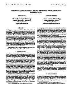
where oˆi is the value of the ith unit of the DBN output layer (each output node is associated to a specific label) and oi is the ground-truth value of the corresponding labeled input data, following the one-hot encoding (i.e. class 1 is coded as “10000”, class 2 as “01000”, etc.). Input values lie between 0 and 1, and they are obtained by normalization of the audio features resulting from the MFCCs extraction and logarithm of energy computation. 4. EXPERIMENTAL RESULTS All the experiments have been performed on a real world dataset, that is available on request, consisting in more than two hours of soccer videos in Italian language. It contains matches of different teams (e.g. city teams such as Barcelona and national teams such as Italy), and different broadcasters (Eurosport, Rai, Tele+) with different speakers of different gender. In fact speakers are usually males, but there are few female commentators in the studio setting that is shown during the break of the match. In particular the audio signal is coded in AC-3 format, with two channels and 44.1 KHz sampling rate. The audio stream has been converted to mono and downsampled to 16 KHz, then divided in windows of 2 seconds for a total of 4065 segments, to extract the audio features. All of these segments have been manually labeled in five different audio events: Silence, Speech Only, Speech Over Crowd, Crowd Only, Excited; the Excited class contains excited speech, excited crowd noise or a combination of them. Fig. 2 shows sample keyframes associated with the audio events. The occurrences of these events in a soccer videos is quite different. In fact, Speech Over Crowd and Excited events are the most

1200

800

400

0

Silence

Speech Only

Speech Over Crowd

Crowd Only

Excited

Fig. 3. Frequency samples for each class in the dataset. Silence

1.0

.00

.00

.00

.00

Speech Only

.00

.92

.08

.00

.00

Speech over Crowd

.00

.01

.75

.02

.22

Crowd Only

.00

.00

.11

.85

.04

Excited

.00

.00

.30

.02

.68

Sil e

Sp e

nc e

Cr Ex ow cit ec ec ed dO ho hO v n nly er ly Cr ow d Sp e

Fig. 4. Confusion matrix of SVM classifier. frequent while, for example, Speech Only events usually occur only during the break of the match. For this reason our dataset is unbalanced. Fig. 3 shows the frequency distribution for each class. Training and test dataset have been taken according to a 3-fold cross-validation. We compare the proposed DBN classification method to SVM, that is widely used in the literature as classification method. The SVM kernel function used is Chi-square, while the trained DBN consists of three hidden layers of logistic units resulting in a 820-800-800-4000-5 structure. In particular, the pre-training process for each layer was of 50 epochs and the fine-training was computed applying early-stopping criterion within 200 epochs. Fig. 4 and Fig. 5 report the confusion matrices for the SVM and DBN classifiers respectively. The overall accuracy for SVM is 74.13% while the DBN has a slightly lower accuracy of 71.67%. These global accuracies are obtained weighting the accuracy of the classes with their cardinality (because of the unbalancing of the dataset). Silence is always correctly classified, followed by the Speech Only. This latter class is particularly interesting since it is related to the sequences that show the commentators in the studio, and thus may be used to segment and classify video shots. Moreover the audio sequences that have been classified as Speech Only may be chosen to perform speech recognition, to add high-level semantic annotation to the video. The Speech Over Crowd is related to ongoing actions while the Excited class is related to highlights such as shots

Fig. 2. Sample keyframes associated to the audio events classified by the system.

Silence

1.0

.00

.00

.00

.00

Speech Only

.00

.86

.14

.00

.00

Speech over Crowd

.00

.01

.74

.02

.23

Crowd Only

.00

.02

.22

.59

.17

Excited

.00

.00

.28

.04

.68

Sil e

nc e

Sp e

ec h

Cr Sp Ex ow ee cit ch ed dO ov On n er ly ly Cr ow d

Fig. 5. Confusion matrix of DBN classifier. on goal, placed kicks near the goal post, penalty kicks, etc. The Crowd Only class is related to shots showing actions but without the speech of commentators. The lower accuracy of DBN is mainly due to the two audio classes that are less represented in the data set, thus we expect that increasing the training set of these two classes may solve the problem. Moreover, DBNs have been introduced very recently and there is an interesting effort in the research community to define RBM layers that deal with continuousvalued input vectors [8]. In fact, the values fed to the RBM (see Sect. 3.1) are obtained through quantization of audio features that are continuous values. Thus, we expect that using the original values, as in the visual domain [13, 11], we can improve the performances. 5. CONCLUSIONS In this paper we have presented a novel method for audio event classification based on the use of a deep belief neural network. The method has been tested on broadcast soccer videos to recognize audio events that are connected to video highlights and types of scenes. The preliminary results show comparable classification results with state-of-theart Chi-square based SVM classifier. Future works will deal with the improvement of classification performances, through the definition of RBM layers that deal with continuous-valued input vectors. Acknowledgements This work is partially supported by the EU IST VidiVideo Project (Contract FP6-045547) and IM3I Project (Contract FP7-222267).

6. REFERENCES [1] D. A. Sadlier and N. E. O’Connor, “Event detection in field sports video using audio-visual features and a support vector machine,” IEEE Trans. on Circuits and Systems for Video Technology, vol. 15, no. 10, 2005. [2] A. Hanjalic, “Adaptive extraction of highlights from a sport video based on excitement modeling,” IEEE Trans. on Multimedia, vol. 7, no. 6, 2005. [3] K. Wickramaratna, M. Chen, S.-C. Chen, and M.-L. Shyu, “Neural network based framework for goal event detection in soccer videos,” in Proc. of ISM, 2005. [4] I. Otsuka, R. Radhakrishnan, M. Siracusa, A. Divakaran, and H. Mishima, “An enhanced video summarization system using audio features for a personal video recorder,” IEEE Trans. on Consumer Elec., vol. 52, no. 1, 2006. [5] H.-G. Kim, J. Jeong, J.-H. Kim, and J.Y. Kim, “Real-time highlight detection in baseball video for TVs with time-shift function,” IEEE Trans. on Consumer Elec., vol. 54, no. 2, 2008. [6] M. Xu, C. Xu, L. Duan, J. Jin, and S. Luo, “Audio keywords generation for sports video analysis,” ACM TOMCCAP, vol. 4, no. 2, 2008. [7] E. G. Hinton, S. Osindero, and Y. Teh, “A fast learning algorithm for deep belief nets,” Neural Computation, vol. 18, 2006. [8] Y. Bengio, P. Lamblin, D. Popovici, and H. Larochelle, “Greedy layer-wise training of deep networks,” in Proc. of NIPS, 2006. [9] E. G. Hinton and R. Salakhutdinov, “Reducing the dimensionality of data with neural networks,” Science, vol. 313, no. 5786, 2006. [10] R. Salakhutdinov and E. G. Hinton, “Semantic hashing,” in Proc. of ACM SIGIR, 2007. [11] E. H¨orster and R. Lienhart, “Deep networks for image retrieval on large-scale databases,” in Proc. of ACM Multimedia, 2008. [12] A. Torralba, R. Fergus, and Y. Weiss, “Small codes and large image databases for recognition,” in Proc. of CVPR, 2008. [13] H. Larochelle, D. Erhan, A. Courville, J. Bergstra, and Y. Bengio, “An empirical evaluation of deep architectures on problems with many factors of variation,” in Proc. of ICML, 2007. [14] Y. Bengio and Y. LeCunn, Large scale kernel machines, chapter Scaling learning algorithms towards AI, MIT Press, 2007. [15] H. G. Kim, N. Moreau, and T. Sikora, MPEG-7 Audio and Beyond: Audio Content Indexing and Retrieval, John Wiley & Sons, 2005.