AN ENSEMBLE OF DEEP NEURAL NETWORKS FOR ... - CiteSeerX

AN ENSEMBLE OF DEEP NEURAL NETWORKS FOR OBJECT TRACKING Xiangzeng Zhou, Lei Xie, Peng Zhang and Yanning Zhang Shaanxi Provincial Key Laboratory of Speech & Image Information Processing (SAIIP), School of Computer Science, Northwestern Polytechnical University, Xi’an, 710072, P. R. China ABSTRACT Object tracking in complex backgrounds with dramatic appearance variations is a challenging problem in computer vision. We tackle this problem by a novel approach that incorporates a deep learning architecture with an on-line AdaBoost framework. Inspired by its multi-level feature learning ability, a stacked denoising autoencoder (SDAE) is used to learn multi-level feature descriptors from a set of auxiliary images. Each layer of the SDAE, representing a different feature space, is subsequently transformed to a discriminative object/background deep neural network (DNN) classifier by adding a classification layer. By an on-line AdaBoost feature selection framework, the ensemble of the DNN classifiers is then updated on-line to robustly distinguish the target from the background. Experiments on an open tracking benchmark show promising results of the proposed tracker as compared with several state-of-the-art approaches. Index Terms— Boosting, deep learning, visual tracking, deep neural network, AdaBoost 1. INTRODUCTION AND RELATED WORKS Object tracking is a fundamental subject in the field of computer vision with a wide range of applications. The chief challenge of object tracking can be attributed to the difficulty in handling the appearance variability of a target object. To deal with this problem, many approaches have been proposed in recent years [1–12]. Early tracking approaches employ static appearance models which are either defined manually or trained initially in the first frame [1, 2]. Unfortunately, these approaches may face difficulties when the tracked targets have heavy intrinsic appearance changes. It has been verified that an adaptive appearance model, evolving with the change of object appearance, brings better performance [3–8]. Many of these approaches adopted a generative model for object representation. In nature, generative approaches were not equipped to distinguish a target from the background [5, 8]. Modeling both the object and the background via discriminative classifiers is an alternative choice in the design of appearance models [7, 9–11]. In this spirit, object tracking has been formulated as a binary classification problem which distinguishes the object of interest from the background via

a classifier, e.g., support vector machines (SVMs) [12, 13]. Specifically, the idea of boosting was adopted to select discriminative features for robust tracking [7, 9]. Boosting is a general method for improving the performance of a learning algorithm by combining several “weak” learning algorithms [14]. In ensemble tracking (ET) [9], an ensemble of weak classifiers was trained on-line to distinguish between the target and the background and a strong classifier was successfully obtained using AdaBoost [15]. Extended from [16], Grabner et al. [7] have proposed an on-line AdaBoost feature selection algorithm to address a real-time tracking task by updating an ensemble of weak classifiers while tracking. This approach was able to cope with appearance changes of the target. Each weak hypothesis was generated according to a different type of hand-crafted feature. Hand-crafted feature descriptors may lead to unrecoverable information loss and which feature is suitable for tracking in different scenarios is still an unsolved problem. Recently, automatic feature extraction using deep learning techniques brings significant performance improvements in many areas. As a typical deep learning architecture, deep neural networks (DNNs) have shown superior performance in tasks such as speech recognition [17] and natural language processing [18]. The deep architecture performs as an automatic feature extractor [19], and each network layer can be considered as a different feature space of the raw data. In more recent years, deep learning techniques have been successfully applied in several computer vision tasks, such as image classification [20], object detection [21, 22] and object tracking [23]. Recently, Wang et al. [23] proposed a novel deep learning tracker (DLT) for robust visual tracking. DLT combines the philosophies behind both generative and discriminative trackers by automatically learning a deep compact image representation using a stacked denoising autoencoder (SDAE) [24]. Promising results have been reported by this deep learning approach. Inspired by the success of on-line AdaBoost and deep learning, in this paper, we propose a novel object tracking approach which combines a family of deep neural network classifiers using on-line AdaBoost. Firstly, we build an off-line unsupervised generic image feature extractor using an SDAE with a considerable amount of natural images. Each layer of the SDAE serves as a different level of feature space, which

is subsequently transformed to a discriminative DNN classifier by adding an additional classification layer. Secondly, we propose an on-line AdaBoost feature selection framework to combine these layered classifiers for on-line updating. Particle filter is used for tracking and the confidence of each particle is provided by the boosting system. Experimental results on an open tracking benchmark [25] show that our tracker is superior to several state-of-the-art trackers and significant performance gain is achieved as compared with the recent DLT tracker [23]. In the next section, we describe the SDAE-based unsupervised image feature descriptor. In Section 3, we present the proposed approach for on-line boosting a family of deep neural networks. Experiments on an open benchmark are shown in Section 4. Finally, we conclude the paper in Section 5. 2. GENERIC IMAGE FEATURE DESCRIPTOR In this section, we describe the unsupervised generic feature learning scheme, which is based on a stacked denoising autoencoder (SDAE). In an idiomatic manner of a learning deep architecture, we first pretrain the SDAE layer-by-layer and fine-tune the whole SDAE subsequently. This process is carried out off-line using one million images randomly selected from the 80-million tiny images dataset [26]. An SDAE is built by stacking several one-layer neural networks, called denoising autoencoders (DAE), which is trained to denoise the corrupted versions of the raw data [24]. Figure 1(A) shows the architecture of a DAE. Consider there are Nt training samples. Let xi denote the original data sample and x ˜i be the corrupted version of xi . For the network, let W and W0 denote the weights of the encoder and decoder, respectively. Similarly, b and b0 refer to the bias terms. A denoising autoencoder is learned by solving the following optimization problem with regularized term min Θ

Nt ∑

kxi − x ˆi k22 + η(kWk2F + kW0 k2F ),

(1)

i=1

where x ˆi = f (W0 hi + b0 ) i

i

h = f (W˜ x + b)

(2) (3)

Here Θ = (W, W0 , b, b0 ) denote the parameters of the network. f (·) is a nonlinear activation function which is typically the logistic sigmoid function. The factor η balances the reconstruction loss and the weight penalty terms, in which k · kF is the Frobenius norm [27]. It has been shown that, by preventing the autoencoder from simply learning the identity mapping, a denoising autoencoder is more effective than the conventional autoencoder in discovering robust features [24]. After the pretraining step, the SDAE is unrolled to form a feedforward neural network, which is fine-tuned using the backpropagation (BP) procedure. According to the configuration suggested in [23], we use a 4-layer network shown in Fig. 1(B) to achieve our learning. In the proposed tracker, an object in each frame is represented

256

...

512

... 1024

...

Encoder

corruption

Decoder 2056

...

1024

(A)

(B)

Fig. 1. (A) DAE architecture (B) SDAE architecture by a 32×32 image patch. Hence, the size of the input layer of SDAE is 1024 corresponding to a vector of 1024 dimensions. To elaborately describe the image structure, a structure with overcomplete filters is deliberatively chosen in the first hidden layer for the purpose of finding an overcomplete basis. Then, the number of units is reduced by half when a new layer is added until there are only 256 hidden units, which serves as the bottleneck of the autoencoder. 3. TRACKING In this section, we describe our on-line boosting DNN tracker. The main idea is to formulate the tracking problem as an online classification task. In Section 2, we have learned an image feature descriptor using an SDAE. Each layer of the SDAE serves as a different feature space of the raw image data. We transform each layer to a discriminative binary classifier by adding an additional sigmoid classification layer on the top of each layer. In the first frame, the object has been provided by a bounding box and the object region is considered as a positive sample, and the negative samples can be extracted from the surrounding background. These positive and negative samples are used to adapt the DNN classifiers via the BP algorithm in several iterations. After that, an on-line boosting feature selection mechanism is used to combine the well-fitted binary classifiers. The tracking is carried out based on a particle filter. In each frame, a set of particles, corresponding to the object candidates, are drawn from an importance distribution. A confidence map of each image region of an object candidate is evaluated by the on-line boosting DNNs system. The region with the maximal confidence is then taken as the new location of the object. Once the object has been detected in current frame, the online boosting system is updated to the possible appearance variation. Similarly, the current object region is regarded as a positive sample and the surrounding regions as negative samples. The whole tracking and updating procedure is repeated once a new frame arrives. 3.1. Particle Filter based Tracking Our tracking process is formulated within a Bayesian framework in which a particle filter [28] is used. Let xt and yt denote the hidden state and observation variables at time t, respectively. The state here is represented by the affine transformation parameters which correspond to translation, scale, aspect ratio, rotation, and skewness. Up to time t − 1, the

+ - ...

Ns training samples Initial importance of the samples λ1:4,1:Ns= 10

hSelector1

hSelector2

DNN1

DNN1

DNN2

update λ1:4,1:Ns

DNN3 DNN4

Repeat for each frame

DNN2 DNN3

DNN1 update λ1:4,1:Ns

...

DNN4

Update Weight α 1

Algorithm 1 On-line Boosting DNNs

hSelectorN

Update Weight α 2

DNN2 DNN3 DNN4 Update Weight α N

Current strong classifer hStrong

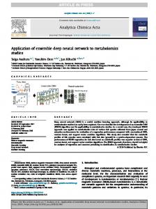
wrong 1: Init: λcorr ˆ0,m = 0.1 n,m,i = 1, λn,m,i = 1, λn,m,i = 10, e 2: for n = 1, 2, ..., N do 3: for m = 1, 2, ..., M do 4: DNNn,m = update(DNNn,m , hXt , Yt i, λ) 5: en,m,i = |DNNn,m (xit ) − yti | (en,m,i ∈ [0, 1]) 6: if en,m,i < 0.5 then corr 7: λcorr n,m,i = λn,m,i + λn,m,i × en,m,i wrong = λ 8: λwrong n,m,i n,m,i + λn,m,i × (1 − en,m,i ) 9: else wrong 10: λwrong n,m,i = λn,m,i + λn,m,i × en,m,i corr corr 11: λn,m,i = λn,m,i + λn,m,i × (1 − en,m,i ) 12: end if wrong λn,m,i wrong

Fig. 2. On-line boosting DNNs.

13:

predicting posterior distribution of xt given all available observations y1:t−1 = {y1 , y2 , ..., yt−1 } is computed as

14: 15: 16: 17:

end for ∑Ns eˆn,m = N1 i=1 en,m,i s m∗ = arg maxm (ˆ en−1,m − eˆn,m ) hsel n = DNNm∗

18:

α = exp (

∫

p(xt |y1:t−1 ) =

p(xt |xt−1 )p(xt−1 |y1:t−1 )dxt−1 .

(4)

Inference to time t, the observation yt is available and the posterior distribution of xt is updated using the Bayesian formulation p(xt |y1:t ) =

p(yt |xt )p(xt |y1:t−1 ) . p(yt |y1:t−1 )

(5)

The job of particle filter is to approximate the posterior p(xt |y1:t ) by a finite set of N samples {xit }i=1,...,N , called particles, associated with normalized importance weights wti . The particles xit are drawn from an importance distribution q(xt |x1:t−1 , y1:t ) and the corresponding weights are updated using i wti = wt−1

p(yt |xit )p(xit |xit−1 ) . q(xt |x1:t−1 , y1:t )

(6)

The importance distribution q(xt |x1:t−1 , y1:t ) is often simplified with first-order Markov assumption to q(xt |xt−1 ), and consequently the weights updating becomes wti = i p(yt |xit ). In our approach, the motion model q(xt |xt−1 ) wt−1 is modeled independently by a normal distribution and the observation model p(yt |xit ) is estimated by an on-line boosting classifier whose output is a kind of confidence measure. 3.2. On-line Boosting DNNs Given a learned image feature descriptor in Section 2, each layer of the SDAE serves as a different level of feature. We build several discriminative binary DNN classifiers by adding a sigmoid layer on the top of each layer of the SDAE, and combine these classifiers using the on-line boosting framework [7]. Specifically, we present a modified version of online AdaBoosting to be more applicable to the DNN classifiers. The modifications include voting weight updating, sample importance weight updating and DNN classifiers updating with weighted samples, as described in Algorithm 1. For the requirement of on-line DNN updating, we carry out the boosting learning process in a batch manner. The framework of the proposed on-line boosting DNN framework is shown in Fig. 2, and the corresponding algorithm pseudo-code is presented in Algorithm 1. Let Xt =

en,m,i =

λn,m,i +λcorr n,m,i

e ˆn−1,m∗ −ˆ en,m∗ e ˆn−1,m∗

)

19: λn,m,i = λn,m,i × en,m,i 20: end for

s {x1t , ..., xN t } denote the Ns training samples associated with labels Yt = {0, 1} at frame t. At the first frame, following the concept of selector in [7], a fixed set of N selectors sel {hsel 1 , ..., hN } is initialized randomly. Once a set of training samples hXt , Yt i arrive at frame t, selectors are updated with respect to the importance weights λ of current samples. In order to update the DNN classifiers with weighted samples, the feedforward error is weighted by multiplying with λ before the BP process. This is done for all samples over each DNN classifier in a batch manner. After that, the error en,m,i is estimated from the weights of correctly and wrongly classiwrong fied examples (λcorr n,m,i and λn,m,i ), where en,m,i is the error of the i-th sample over the m-th DNN classifier in the n-th selector. Then, the selector hsel n selects one DNN classifier with the maximal error reducing margin in average. Subsequently, the voting weight αn and the importance weight λ are updated, and then the algorithm moves on to the next selector. This process is repeated for all selectors. Finally, a final strong classifier hstrong is obtained by a linear combination of selectors to serve as a confidence measure for the particle filter.

4. EXPERIMENTS 4.1. Experimental Settings We compare our proposed approach with some state-ofart trackers over 8 video sequences on a standard benchmark [25]. For off-line training of the SDAE, we follow the parameter configuration of the recent DLT tracker [23]. The momentum parameter is set to 0.9. The mini-batch size is set to 100 for off-line training and to 10 for on-line updating. For the on-line tracking system, we draw 1000 particles for the particle filter. The number N of selectors is set to 5 and the number M of DNN classifiers is 4.

Table 1. Comparison of 7 trackers on 8 video sequences. The first number denotes the success rate in percentage and the number in brackets denotes the central-pixel error in pixels. Sylvester

Coke

Woman

Girl

Car4

David3

David

Bolt

CT [29] DLT [23] IVT [5] L1T [30] MIL [3] MTT [31] Ours

82.8(8.6) 84.1(7.0) 67.6(34.2) 42.8(26.2) 54.6(15.2) 82.3(7.6) 91.9(6.6)

9.3(40.5) 59.8(28.4) 13.1(83.0) 20.0(50.4) 11.7(46.7) 61.5(30.0) 69.1(26.6)

17.0(115.0) 21.1(144.1) 19.6(174.1) 20.9(128.7) 20.0(127.3) 21.1(136.8) 86.4(5.5)

17.8(18.9) 95.2(3.0) 18.6(22.5) 97.0(2.8) 29.4(13.7) 93.2(4.3) 89.0(3.2)

27.5(86.0) 100(2.6) 100(2.1) 30.0(77.0) 27.6(50.8) 31.1(22.3) 100(3.3)

34.9(88.7) 33.3(104.8) 63.5(52.0) 45.6(90.0) 68.3(29.7) 10.3(341.3) 54.8(66.0)

42.7(10.5) 82.0(6.6) 79.4(4.8) 69.2(14.0) 22.9(16.9) 28.9(33.1) 84.7(6.2)

0.6(363.8) 2.3(388.1) 1.4(397.0) 1.1(408.4) 1.1(393.5) 1.1(408.6) 24.5(111.6)

CT [29] DLT [23] IVT [5] L1T [30] MIL [3] MTT [31] Ours

1132-OPR SUCCESS 911-OPR 597-OPR 717-IV 1138-OPR SUCCESS

22-IV 177-FM 39-OCC 82-OPR 70-FM 190-OCC 177-FM

95-DEF 119-OCC 110-OCC 118-OCC 119-OCC 119-OCC SUCCESS

98-OPR SUCCESS 91-OPR SUCCESS 98-OPR SUCCESS SUCCESS

186-IV SUCCESS SUCCESS 199-SV 199-SV 207-SV SUCCESS

83-OCC 82-OCC 190-OCC 118-OPR 100-DEF 27-DEF 82-OCC

406-IV SUCCESS 94-DEF SUCCESS SUCCESS 153-OPR SUCCESS

3-DEF 9-DEF 6-DEF 5-DEF 5-DEF 5-DEF 119-DEF

4.2. Quantitative and Qualitative Performance For quantitative comparison, we use two standard metrics: success rate and central-pixel error. Both the tracking result and the labeled groundtruth are represented by a bounding box, respectively. In each frame, once the overlap percentage of the two bounding boxes is larger than 50% against the entire union box, the tracking is considered as a successful case. The central-pixel error is defined as the Euclidean distance between the centers of the two bounding boxes. Table 1 over 8 typical #300 #125summarizes the performances of the 7 trackers video sequences in the top half. The best results are highlighted in bold font. It’s clearly observed that our proposed approach is superior to other methods on 6 video sequences. For the other 2 video sequences, our method is also among the best three methods. Figure 3 shows some tracking results. We have analyzed the robustness of the 7 trackers against some common problems defined in [25]: illumination vari#351 non-rigid object #410 ation (IV), partial or full occlusion (OCC), deformation (DEF), fast motion (FM) and out-of-plane rotation (OPR). Each entity in the bottom half of Table 1 means that a tracker fails in which frame due to what reason. The SUCCESS means the tracker finished with tracking success, but may suffer several unsuccessful cases in the middle. It’s clearly observed that our tracker and the DLT tracker win the most and second most successful tracking, respectively. In the #1000woman sequence, our tracker doesn’t#15 drift whilst most trackers fail due to severe occlusions. The Bolt is a challenging sequence on which most trackers fail in early frames due to severe deformation. However, our tracker continues tracking till frame 119. In the David3 sequence, our tracker fails because of full occlusion. Fast motion (FM) also causes our tracker’s failure as shown in the Coke sequence. #300

#125

#1000

#410

#1000

#300

#125

#410

#87

#134

#1000

#351

#410

#125

family of discriminative DNN classifiers is then built from the different layers of the SDAE. After that, these classifiers are combined with an alternative version of the on-line boosting to facilitate the object/background classification. Promising results have been achieved. We believe that the key to the success of our approach lies in two-fold. First, the deep learning architecture can automatically learn useful generic image features in different levels. Second, which level of feature is most suitable for appearance modeling is further automatically decided by boosting. In the future, we plan #87 to use a convolutional neural network (CNN) which recently has shown better capability of extracting image features [20]. Currently, without aiding with GPU our tracker suffers a little time-consuming DNN updating, and this would be our next work to reduce computation cost with GPU. We also plan to investigate how the depth of the deep architecture affects the tracking performance. #134

#300

#1000

#15

#87

#87

#134

#15 #410

#125

#410

#125

2

#351

#134

#300

#351

1.5 Ours

#134

#300 CT

IVT

L1APG

MIL

MTT

DLT

0 0

Sylvester

Coke

2

#300

#87 1.5 Ours

CT

IVT

#1000

#410

#1000 #87

#410

L1APG

MIL

Woman

0.5

#15

1

Girl

#15

MTT

1.5

2

#351

2 1.5 Ours 1.5 1 Ours

DLT

1

Car4

1.5

0.5

#134

Ours

1

1.5

David3

#1000 #1000

#134

CT

0.5 0 0 0 0

2

IVT

David

L1T

Bolt #15

#15

MIL

MTT

DLT

1

Fig. 3. Comparison of 7 trackers on several key frames in terms of the0.5bounding box. #15

CT

CT

1 0.5

200

#351

2

#351

0.5

02 0 1.5 Ours

2 0.5

1

1.5

2

6. ACKNOWLEDGMENT 1.5 IVT Ours

CT

1

5. CONCLUSIONS AND FUTURE WORK In this paper, we have presented a novel object tracker by integrating the deep learning technique with the on-line boosting framework. We first use a stacked denoising autoencoder (SDAE) to learn a multi-level image feature descriptor. A

#300

#300

0.5

#351

#410

#351 #125

#125

1

#15

#125

#87

L1APG CT

IVT MIL

L1APG MTT

DLT MIL

MTT

DLT

1

This work was supported by the National Natural Science Foundation of China (61175018, 61301194), the Fok Ying Tung Education Foundation (131059) and the doctoral program of High Education of China (No. 20126102120055) approved by the Ministry of Education, China. 0.5

0.5

0

0

0

0.5

0 1

0.51.5

1 2

1.5

2

0.5

0.5

References [1] Amit Adam, Ehud Rivlin, and Ilan Shimshoni, “Robust fragments-based tracking using the integral histogram,” in CVPR ’06, 2006, vol. 1, pp. 798–805. [2] Dorin Comaniciu, Visvanathan Ramesh, and Peter Meer, “Real-time tracking of non-rigid objects using mean shift,” in CVPR ’00, 2000, vol. 2, pp. 142–149. [3] Boris Babenko, Ming-Hsuan Yang, and Serge Belongie, “Visual tracking with online multiple instance learning,” in CVPR ’09, 2009, pp. 983–990. [4] Junseok Kwon and Kyoung Mu Lee, “Visual tracking decomposition,” in CVPR ’10, 2010, pp. 1269–1276. [5] David A Ross, Jongwoo Lim, Ruei-Sung Lin, and MingHsuan Yang, “Incremental learning for robust visual tracking,” IJCV ’08, vol. 77, pp. 125–141, 2008. [6] Helmut Grabner, Christian Leistner, and Horst Bischof, “Semi-supervised on-line boosting for robust tracking,” in ECCV ’08, 2008, pp. 234–247. [7] Helmut Grabner, Michael Grabner, and Horst Bischof, “Real-time tracking via on-line boosting.,” in BMVC ’06, 2006, vol. 1, p. 6. [8] David Ross, Jongwoo Lim, and Ming-Hsuan Yang, “Adaptive probabilistic visual tracking with incremental subspace update,” in ECCV ’04, 2004, pp. 470–482. [9] Shai Avidan, “Ensemble tracking,” PAMI ’07, vol. 29, pp. 261–271, 2007. [10] Jianyu Wang, Xilin Chen, and Wen Gao, “Online selecting discriminative tracking features using particle filter,” in CVPR ’05, 2005, vol. 2, pp. 1037–1042. [11] Robert T Collins, Yanxi Liu, and Marius Leordeanu, “Online selection of discriminative tracking features,” PAMI ’05, vol. 27, pp. 1631–1643, 2005. [12] Oliver Williams, Andrew Blake, and Roberto Cipolla, “Sparse bayesian learning for efficient visual tracking,” PAMI ’05, vol. 27, pp. 1292–1304, 2005. [13] Shai Avidan, “Support vector tracking,” PAMI ’04, vol. 26, pp. 1064–1072, 2004. [14] Nikunj C Oza, “Online bagging and boosting,” in IEEE international conference on Systems, Man and Cybernetics, 2005, vol. 3, pp. 2340–2345. [15] Yoav Freund, Robert E Schapire, et al., “Experiments with a new boosting algorithm,” in ICML ’96, 1996, vol. 96, pp. 148–156. [16] Omar Javed, Saad Ali, and Mubarak Shah, “Online detection and classification of moving objects using progressively improving detectors,” in CVPR ’05, 2005, vol. 1, pp. 696–701. [17] George E Dahl, Dong Yu, Li Deng, and Alex Acero, “Context-dependent pre-trained deep neural networks for large-vocabulary speech recognition,” IEEE Trans.

[18]

[19]

[20]

[21]

[22]

[23]

[24]

[25] [26]

[27]

[28]

[29]

[30]

[31]

on Audio, Speech, and Language Processing, vol. 20, pp. 30–42, 2012. Ronan Collobert and Jason Weston, “A unified architecture for natural language processing: Deep neural networks with multitask learning,” in ICML ’08, 2008, pp. 160–167. Yoshua Bengio, “Learning deep architectures for ai,” Foundations and Trends in Machine Learning, vol. 2, pp. 1–127, 2009. Alex Krizhevsky, Ilya Sutskever, and Geoff Hinton, “Imagenet classification with deep convolutional neural networks,” in Advances in Neural Information Processing Systems 25, 2012, pp. 1106–1114. Brody Huval, Adam Coates, and Andrew Ng, “Deep learning for class-generic object detection,” arXiv preprint arXiv:1312.6885, 2013. Ross Girshick, Jeff Donahue, Trevor Darrell, and Jitendra Malik, “Rich feature hierarchies for accurate object detection and semantic segmentation,” arXiv preprint arXiv:1311.2524, 2013. Naiyan Wang and Dit-Yan Yeung, “Learning a deep compact image representation for visual tracking,” in NIPS ’13, 2013, pp. 809–817. Pascal Vincent, Hugo Larochelle, Isabelle Lajoie, Yoshua Bengio, and Pierre-Antoine Manzagol, “Stacked denoising autoencoders: Learning useful representations in a deep network with a local denoising criterion,” The Journal of Machine Learning Research, vol. 9999, pp. 3371–3408, 2010. Yi Wu, Jongwoo Lim, and Ming-Hsuan Yang, “Online object tracking: A benchmark,” in CVPR ’13, 2013. Antonio Torralba, Robert Fergus, and William T Freeman, “80 million tiny images: A large data set for nonparametric object and scene recognition,” PAMI ’08, vol. 30, pp. 1958–1970, 2008. Gene H. Golub and Charles F. Van Loan, Matrix Computations (3rd Ed.), Johns Hopkins University Press, Baltimore, MD, USA, 1996. M Sanjeev Arulampalam, Simon Maskell, Neil Gordon, and Tim Clapp, “A tutorial on particle filters for online nonlinear/non-gaussian bayesian tracking,” IEEE Trans. on Signal Processing, vol. 50, pp. 174–188, 2002. Kaihua Zhang, Lei Zhang, and Ming-Hsuan Yang, “Real-time compressive tracking,” in ECCV ’12, pp. 864–877. 2012. Boris Babenko, Ming-Hsuan Yang, and Serge Belongie, “Robust object tracking with online multiple instance learning,” PAMI ’11, vol. 33, pp. 1619–1632, 2011. Tianzhu Zhang, Bernard Ghanem, Si Liu, and Narendra Ahuja, “Robust visual tracking via multi-task sparse learning,” in CVPR ’12, 2012, pp. 2042–2049.