DeepFM: A Factorization-Machine based Neural Network for CTR Prediction
arXiv:1703.04247v1 [cs.IR] 13 Mar 2017
Huifeng Guo∗1 , Ruiming Tang2 , Yunming Ye†1 , Zhenguo Li2 , Xiuqiang He2 1 Shenzhen Graduate School, Harbin Institute of Technology, China 2 Noah’s Ark Research Lab, Huawei, China 1
[email protected],
[email protected] 2 {tangruiming, li.zhenguo, hexiuqiang}@huawei.com Abstract Learning sophisticated feature interactions behind user behaviors is critical in maximizing CTR for recommender systems. Despite great progress, existing methods seem to have a strong bias towards low- or high-order interactions, or require expertise feature engineering. In this paper, we show that it is possible to derive an end-to-end learning model that emphasizes both low- and highorder feature interactions. The proposed model, DeepFM, combines the power of factorization machines for recommendation and deep learning for feature learning in a new neural network architecture. Compared to the latest Wide & Deep model from Google, DeepFM has a shared input to its “wide” and “deep” parts, with no need of feature engineering besides raw features. Comprehensive experiments are conducted to demonstrate the effectiveness and efficiency of DeepFM over the existing models for CTR prediction, on both benchmark data and commercial data.
1
Introduction
The prediction of click-through rate (CTR) is critical in recommender system, where the task is to estimate the probability a user will click on a recommended item. In many recommender systems the goal is to maximize the number of clicks, and so the items returned to a user can be ranked by estimated CTR; while in other application scenarios such as online advertising it is also important to improve revenue, and so the ranking strategy can be adjusted as CTR×bid across all candidates, where “bid” is the benefit the system receives if the item is clicked by a user. In either case, it is clear that the key is in estimating CTR correctly. It is important for CTR prediction to learn implicit feature interactions behind user click behaviors. By our study in a mainstream apps market, we found that people often download apps for food delivery at meal-time, suggesting that the (order-2) interaction between app category and time-stamp ∗ This work is done when Huifeng Guo worked as intern at Noah’s Ark Research Lab, Huawei. † Corresponding Author.
Figure 1: Wide & deep architecture of DeepFM. The wide and deep component share the same input raw feature vector, which enables DeepFM to learn low- and high-order feature interactions simultaneously from the input raw features.
can be used as a signal for CTR. As a second observation, male teenagers like shooting games and RPG games, which means that the (order-3) interaction of app category, user gender and age is another signal for CTR. In general, such interactions of features behind user click behaviors can be highly sophisticated, where both low- and high-order feature interactions should play important roles. According to the insights of the Wide & Deep model [Cheng et al., 2016] from google, considering low- and high-order feature interactions simultaneously brings additional improvement over the cases of considering either alone. The key challenge is in effectively modeling feature interactions. Some feature interactions can be easily understood, thus can be designed by experts (like the instances above). However, most other feature interactions are hidden in data and difficult to identify a priori (for instance, the classic association rule “diaper and beer” is mined from data, instead of discovering by experts), which can only be captured automatically by machine learning. Even for easy-to-understand interactions, it seems unlikely for experts to model them exhaustively, especially when the number of features is large. Despite their simplicity, generalized linear models, such as FTRL [McMahan et al., 2013], have shown decent performance in practice. However, a linear model lacks the ability to learn feature interactions, and a common practice is to manually include pairwise feature interactions in its feature vector. Such a method is hard to generalize to model high-order feature interactions or those never or rarely appear in the training data [Rendle, 2010]. Factorization Machines
(FM) [Rendle, 2010] model pairwise feature interactions as inner product of latent vectors between features and show very promising results. While in principle FM can model high-order feature interaction, in practice usually only order2 feature interactions are considered due to high complexity. As a powerful approach to learning feature representation, deep neural networks have the potential to learn sophisticated feature interactions. Some ideas extend CNN and RNN for CTR predition [Liu et al., 2015; Zhang et al., 2014], but CNN-based models are biased to the interactions between neighboring features while RNN-based models are more suitable for click data with sequential dependency. [Zhang et al., 2016] studies feature representations and proposes Factorization-machine supported Neural Network (FNN). This model pre-trains FM before applying DNN, thus limited by the capability of FM. Feature interaction is studied in [Qu et al., 2016], by introducing a product layer between embedding layer and fully-connected layer, and proposing the Product-based Neural Network (PNN). As noted in [Cheng et al., 2016], PNN and FNN, like other deep models, capture little low-order feature interactions, which are also essential for CTR prediction. To model both lowand high-order feature interactions, [Cheng et al., 2016] proposes an interesting hybrid network structure (Wide & Deep) that combines a linear (“wide”) model and a deep model. In this model, two different inputs are required for the “wide part” and “deep part”, respectively, and the input of “wide part” still relies on expertise feature engineering. One can see that existing models are biased to low- or highorder feature interaction, or rely on feature engineering. In this paper, we show it is possible to derive a learning model that is able to learn feature interactions of all orders in an endto-end manner, without any feature engineering besides raw features. Our main contributions are summarized as follows:
clicked the item, and y = 0 otherwise). χ may include categorical fields (e.g., gender, location) and continuous fields (e.g., age). Each categorical field is represented as a vector of one-hot encoding, and each continuous field is represented as the value itself, or a vector of one-hot encoding after discretization. Then, each instance is converted to (x, y) where x = [xf ield1 , xf ield2 , ..., xf iledj , ..., xf ieldm ] is a ddimensional vector, with xf ieldj being the vector representation of the j-th field of χ. Normally, x is high-dimensional and extremely sparse. The task of CTR prediction is to build a prediction model yˆ = CT R model(x) to estimate the probability of a user clicking a specific app in a given context.
2.1
DeepFM
We aim to learn both low- and high-order feature interactions. To this end, we propose a Factorization-Machine based neural network (DeepFM). As depicted in Figure 11 , DeepFM consists of two components, FM component and deep component, that share the same input. For feature i, a scalar wi is used to weigh its order-1 importance, a latent vector Vi is used to measure its impact of interactions with other features. Vi is fed in FM component to model order-2 feature interactions, and fed in deep component to model high-order feature interactions. All parameters, including wi , Vi , and the network parameters (W (l) , b(l) below) are trained jointly for the combined prediction model: yˆ = sigmoid(yF M + yDN N ),
(1)
where yˆ ∈ (0, 1) is the predicted CTR, yF M is the output of FM component, and yDN N is the output of deep component. FM Component
• We propose a new neural network model DeepFM (Figure 1) that integrates the architectures of FM and deep neural networks (DNN). It models low-order feature interactions like FM and models high-order feature interactions like DNN. Unlike the wide & deep model [Cheng et al., 2016], DeepFM can be trained endto-end without any feature engineering. • DeepFM can be trained efficiently because its wide part and deep part, unlike [Cheng et al., 2016], share the same input and also the embedding vector. In [Cheng et al., 2016], the input vector can be of huge size as it includes manually designed pairwise feature interactions in the input vector of its wide part, which also greatly increases its complexity. • We evaluate DeepFM on both benchmark data and commercial data, which shows consistent improvement over existing models for CTR prediction.
2
Our Approach
Suppose the data set for training consists of n instances (χ, y), where χ is an m-fields data record usually involving a pair of user and item, and y ∈ {0, 1} is the associated label indicating user click behaviors (y = 1 means the user
Figure 2: The architecture of FM. The FM component is a factorization machine, which is proposed in [Rendle, 2010] to learn feature interactions for recommendation. Besides a linear (order-1) interactions among features, FM models pairwise (order-2) feature interactions as inner product of respective feature latent vectors. 1
In all Figures of this paper, a Normal Connection in black refers to a connection with weight to be learned; a Weight-1 Connection, red arrow, is a connection with weight 1 by default; Embedding, blue dashed arrow, means a latent vector to be learned; Addition means adding all input together; Product, including Innerand Outer-Product, means the output of this unit is the product of two input vector; Sigmoid Function is used as the output function in CTR prediction; Activation Functions, such as relu and tanh, are used for non-linearly transforming the signal.
It can capture order-2 feature interactions much more effectively than previous approaches especially when the dataset is sparse. In previous approaches, the parameter of an interaction of features i and j can be trained only when feature i and feature j both appear in the same data record. While in FM, it is measured via the inner product of their latent vectors Vi and Vj . Thanks to this flexible design, FM can train latent vector Vi (Vj ) whenever i (or j) appears in a data record. Therefore, feature interactions, which are never or rarely appeared in the training data, are better learnt by FM. As Figure 2 shows, the output of FM is the summation of an Addition unit and a number of Inner Product units: yF M = hw, xi +
d X
d X
hVi , Vj i xj1 · xj2 ,
(2)
j1 =1 j2 =j1 +1
where w ∈ Rd and Vi ∈ Rk (k is given)2 . The Addition unit (hw, xi) reflects the importance of order-1 features, and the Inner Product units represent the impact of order-2 feature interactions. Deep Component
Figure 3: The architecture of DNN. The deep component is a feed-forward neural network, which is used to learn high-order feature interactions. As shown in Figure 3, a data record (a vector) is fed into the neural network. Compared to neural networks with image [He et al., 2016] or audio [Boulanger-Lewandowski et al., 2013] data as input, which is purely continuous and dense, the input of CTR prediction is quite different, which requires a new network architecture design. Specifically, the raw feature input vector for CTR prediction is usually highly sparse3 , super high-dimensional4 , categorical-continuous-mixed, and grouped in fields (e.g., gender, location, age). This suggests an embedding layer to compress the input vector to a lowdimensional, dense real-value vector before further feeding into the first hidden layer, otherwise the network can be overwhelming to train. Figure 4 highlights the sub-network structure from the input layer to the embedding layer. We would like to point out the two interesting features of this network structure: 1) while the lengths of different input field vectors can be different, 2
We omit a constant offset for simplicity. Only one entry is non-zero for each field vector. 4 E.g., in an app store of billion users, the one field vector for user ID is already of billion dimensions. 3
Figure 4: The structure of the embedding layer their embeddings are of the same size (k); 2) the latent feature vectors (V ) in FM now server as network weights which are learned and used to compress the input field vectors to the embedding vectors. In [Zhang et al., 2016], V is pre-trained by FM and used as initialization. In this work, rather than using the latent feature vectors of FM to initialize the networks as in [Zhang et al., 2016], we include the FM model as part of our overall learning architecture, in addition to the other DNN model. As such, we eliminate the need of pre-training by FM and instead jointly train the overall network in an end-to-end manner. Denote the output of the embedding layer as: a(0) = [e1 , e2 , ..., em ],
(3)
where ei is the embedding of i-th field and m is the number of fields. Then, a(0) is fed into the deep neural network, and the forward process is: a(l+1) = σ(W (l) a(l) + b(l) ), (4) (l) where l is the layer depth and σ is an activation function. a , W (l) , b(l) are the output, model weight, and bias of the l-th layer. After that, a dense real-value feature vector is generated, which is finally fed into the sigmoid function for CTR prediction: yDN N = σ(W |H|+1 · aH + b|H|+1 ), where |H| is the number of hidden layers. It is worth pointing out that FM component and deep component share the same feature embedding, which brings two important benefits: 1) it learns both low- and high-order feature interactions from raw features; 2) there is no need for expertise feature engineering of the input, as required in Wide & Deep [Cheng et al., 2016].
2.2
Relationship with the other Neural Networks
Inspired by the enormous success of deep learning in various applications, several deep models for CTR prediction are developed recently. This section compares the proposed DeepFM with existing deep models for CTR prediction. FNN: As Figure 5 (left) shows, FNN is a FM-initialized feedforward neural network [Zhang et al., 2016]. The FM pretraining strategy results in two limitations: 1) the embedding parameters might be over affected by FM; 2) the efficiency is reduced by the overhead introduced by the pre-training stage. In addition, FNN captures only high-order feature interactions. In contrast, DeepFM needs no pre-training and learns both high- and low-order feature interactions. PNN: For the purpose of capturing high-order feature interactions, PNN imposes a product layer between the embedding layer and the first hidden layer [Qu et al., 2016]. According to different types of product operation, there are three variants: IPNN, OPNN, and PNN∗, where IPNN is based on inner product of vectors, OPNN is based on outer product, and PNN∗ is based on both inner and outer products.
Figure 5: The architectures of existing deep models for CTR prediction: FNN, PNN, Wide & Deep Model Table 1: Comparison of deep models for CTR prediction FNN PNN Wide & Deep DeepFM
No Pre-training × √ √ √
High-order Features √ √ √ √
Low-order Features × × √ √
No Feature Engineering √ √ × √
3
Experiments
In this section, we compare our proposed DeepFM and the other state-of-the-art models empirically. The evaluation result indicates that our proposed DeepFM is more effective than any other state-of-the-art model and the efficiency of DeepFM is comparable to the best ones among the others.
3.1 To make the computation more efficient, the authors proposed the approximated computations of both inner and outer products: 1) the inner product is approximately computed by eliminating some neurons; 2) the outer product is approximately computed by compressing m k-dimensional feature vectors to one k-dimensional vector. However, we find that the outer product is less reliable than the inner product, since the approximated computation of outer product loses much information that makes the result unstable. Although inner product is more reliable, it still suffers from high computational complexity, because the output of the product layer is connected to all neurons of the first hidden layer. Different from PNN, the output of the product layer in DeepFM only connects to the final output layer (one neuron). Like FNN, all PNNs ignore low-order feature interactions. Wide & Deep: Wide & Deep (Figure 5 (right)) is proposed by Google to model low- and high-order feature interactions simultaneously. As shown in [Cheng et al., 2016], there is a need for expertise feature engineering on the input to the “wide” part (for instance, cross-product of users’ install apps and impression apps in app recommendation). In contrast, DeepFM needs no such expertise knowledge to handle the input by learning directly from the input raw features. A straightforward extension to this model is replacing LR by FM (we also evaluate this extension in Section 3). This extension is similar to DeepFM, but DeepFM shares the feature embedding between the FM and deep component. The sharing strategy of feature embedding influences (in backpropagate manner) the feature representation by both lowand high-order feature interactions, which models the representation more precisely.
Datasets We evaluate the effectiveness and efficiency of our proposed DeepFM on the following two datasets. 1) Criteo Dataset: Criteo dataset 5 includes 45 million users’ click records. There are 13 continuous features and 26 categorical ones. We split the dataset randomly into two parts: 90% is for training, while the rest 10% is for testing. 2) Company∗ Dataset: In order to verify the performance of DeepFM in real industrial CTR prediction, we conduct experiment on Company∗ dataset. We collect 7 consecutive days of users’ click records from the game center of the Company∗ App Store for training, and the next 1 day for testing. There are around 1 billion records in the whole collected dataset. In this dataset, there are app features (e.g., identification, category, and etc), user features (e.g., user’s downloaded apps, and etc), and context features (e.g., operation time, and etc). Evaluation Metrics We use two evaluation metrics in our experiments: AUC (Area Under ROC) and Logloss (cross entropy). Model Comparison We compare 9 models in our experiments: LR, FM, FNN, PNN (three variants), Wide & Deep, and DeepFM. In the Wide & Deep model, for the purpose of eliminating feature engineering effort, we also adapt the original Wide & Deep model by replacing LR by FM as the wide part. In order to distinguish these two variants of Wide & Deep, we name them LR & DNN and FM & DNN, respectively.6 Parameter Settings To evaluate the models on Criteo dataset, we follow the parameter settings in [Qu et al., 2016] for FNN and PNN: (1) 5
Summarizations: To summarize, the relationship between DeepFM and the other deep models in four aspects is presented in Table 1. As can be seen, DeepFM is the only model that requires no pre-training and no feature engineering, and captures both low- and high-order feature interactions.
Experiment Setup
http://labs.criteo.com/downloads/2014-kaggle-displayadvertising-challenge-dataset/ 6 We do not use the Wide & Deep API released by Google, as the efficiency of that implementation is very low. We implement Wide & Deep by ourselves by simplifying it with shared optimizer for both deep and wide part.
dropout: 0.5; (2) network structure: 400-400-400; (3) optimizer: Adam; (4) activation function: tanh for IPNN, relu for other deep models. To be fair, our proposed DeepFM uses the same setting. The optimizers of LR and FM are FTRL and Adam respectively, and the latent dimension of FM is 10. To achieve the best performance for each individual model on Company∗ dataset, we conducted carefully parameter study, which is discussed in Section 3.3.
3.2
DeepFM outperforms the models that learn high- and low-order feature interactions using separate feature embeddings (namely, LR & DNN and FM & DNN). Compared to these two models, DeepFM achieves more than 0.48% and 0.33% in terms of AUC (0.61% and 0.66% in terms of Logloss) on Company∗ and Criteo datasets. Table 2: Performance on CTR prediction.
Performance Evaluation
In this section, we evaluate the models listed in Section 3.1 on the two datasets to compare their effectiveness and efficiency. Efficiency Comparison The efficiency of deep learning models is important to realworld applications. We compare the efficiency of different models on Criteo dataset by the following formula: |training time of deep CT R model| . The results are shown in |training time of LR| Figure 6, including the tests on CPU (left) and GPU (right), where we have the following observations: 1) pre-training of FNN makes it less efficient; 2) Although the speed up of IPNN and PNN∗ on GPU is higher than the other models, they are still computationally expensive because of the inefficient inner product operations; 3) The DeepFM achieves almost the most efficient in both tests.
Figure 6: Time comparison. Effectiveness Comparison The performance for CTR prediction of different models on Criteo dataset and Company∗ dataset is shown in Table 2, where we have the following observations: • Learning feature interactions improves the performance of CTR prediction model. This observation is from the fact that LR (which is the only model that does not consider feature interactions) performs worse than the other models. As the best model, DeepFM outperforms LR by 0.86% and 4.18% in terms of AUC (1.15% and 5.60% in terms of Logloss) on Company∗ and Criteo datasets. • Learning high- and low-order feature interactions simultaneously and properly improves the performance of CTR prediction model. DeepFM outperforms the models that learn only low-order feature interactions (namely, FM) or high-order feature interactions (namely, FNN, IPNN, OPNN, PNN∗). Compared to the second best model, DeepFM achieves more than 0.37% and 0.25% in terms of AUC (0.42% and 0.29% in terms of Logloss) on Company∗ and Criteo datasets. • Learning high- and low-order feature interactions simultaneously while sharing the same feature embedding for high- and low-order feature interactions learning improves the performance of CTR prediction model.
LR FM FNN IPNN OPNN PNN∗ LR & DNN FM & DNN DeepFM
Company∗ AUC LogLoss 0.8640 0.02648 0.8678 0.02633 0.8683 0.02629 0.8664 0.02637 0.8658 0.02641 0.8672 0.02636 0.8673 0.02634 0.8661 0.02640 0.8715 0.02618
Criteo AUC LogLoss 0.7686 0.47762 0.7892 0.46077 0.7963 0.45738 0.7972 0.45323 0.7982 0.45256 0.7987 0.45214 0.7981 0.46772 0.7850 0.45382 0.8007 0.45083
Overall, our proposed DeepFM model beats the competitors by more than 0.37% and 0.42% in terms of AUC and Logloss on Company∗ dataset, respectively. In fact, a small improvement in offline AUC evaluation is likely to lead to a significant increase in online CTR. As reported in [Cheng et al., 2016], compared with LR, Wide & Deep improves AUC by 0.275% (offline) and the improvement of online CTR is 3.9%. The daily turnover of Company∗’s App Store is millions of dollars, therefore even several percents lift in CTR brings extra millions of dollars each year.
3.3
Hyper-Parameter Study
We study the impact of different hyper-parameters of different deep models, on Company∗ dataset. The order is: 1) activation functions; 2) dropout rate; 3) number of neurons per layer; 4) number of hidden layers; 5) network shape. Activation Function According to [Qu et al., 2016], relu and tanh are more suitable for deep models than sigmoid. In this paper, we compare the performance of deep models when applying relu and tanh. As shown in Figure 7, relu is more appropriate than tanh for all the deep models, except for IPNN. Possible reason is that relu induces sparsity.
Figure 7: AUC and Logloss comparison of activation functions. Dropout Dropout [Srivastava et al., 2014] refers to the probability that a neuron is kept in the network. Dropout is a regularization technique to compromise the precision and the complexity of the neural network. We set the dropout to be 1.0, 0.9, 0.8, 0.7,
0.6, 0.5. As shown in Figure 8, all the models are able to reach their own best performance when the dropout is properly set (from 0.6 to 0.9). The result shows that adding reasonable randomness to model can strengthen model’s robustness.
200-300), decreasing (300-200-100), and diamond (150-300150). As we can see from Figure 11, the “constant” network shape is empirically better than the other three options, which is consistent with previous studies [Larochelle et al., 2009].
Figure 11: AUC and Logloss comparison of network shape.
Figure 8: AUC and Logloss comparison of dropout. Number of Neurons per Layer When other factors remain the same, increasing the number of neurons per layer introduces complexity. As we can observe from Figure 9, increasing the number of neurons does not always bring benefit. For instance, DeepFM performs stably when the number of neurons per layer is increased from 400 to 800; even worse, OPNN performs worse when we increase the number of neurons from 400 to 800. This is because an over-complicated model is easy to overfit. In our dataset, 200 or 400 neurons per layer is a good choice.
Figure 9: AUC and Logloss comparison of number of neurons. Number of Hidden Layers As presented in Figure 10, increasing number of hidden layers improves the performance of the models at the beginning, however, their performance is degraded if the number of hidden layers keeps increasing. This phenomenon is also because of overfitting.
4
In this paper, a new deep neural network is proposed for CTR prediction. The most related domains are CTR prediction and deep learning in recommender system. In this section, we discuss related work in these two domains. CTR prediction plays an important role in recommender system [Richardson et al., 2007; Juan et al., 2016; McMahan et al., 2013]. Besides generalized linear models and FM, a few other models are proposed for CTR prediction, such as tree-based model [He et al., 2014], tensor based model [Rendle and Schmidt-Thieme, 2010], support vector machine [Chang et al., 2010], and bayesian model [Graepel et al., 2010]. The other related domain is deep learning in recommender systems. In Section 1 and Section 2.2, several deep learning models for CTR prediction are already mentioned, thus we do not discuss about them here. Several deep learning models are proposed in recommendation tasks other than CTR prediction (e.g., [Covington et al., 2016; Salakhutdinov et al., 2007; van den Oord et al., 2013; Wu et al., 2016; Zheng et al., 2016; Wu et al., 2017; Zheng et al., 2017]). [Salakhutdinov et al., 2007; Sedhain et al., 2015; Wang et al., 2015] propose to improve Collaborative Filtering via deep learning. The authors of [Wang and Wang, 2014; van den Oord et al., 2013] extract content feature by deep learning to improve the performance of music recommendation. [Chen et al., 2016] devises a deep learning network to consider both image feature and basic feature of display adverting. [Covington et al., 2016] develops a two-stage deep learning framework for YouTube video recommendation.
5
Figure 10: AUC and Logloss comparison of number of layers. Network Shape We test four different network shapes: constant, increasing, decreasing, and diamond. When we change the network shape, we fix the number of hidden layers and the total number of neurons. For instance, when the number of hidden layers is 3 and the total number of neurons is 600, then four different shapes are: constant (200-200-200), increasing (100-
Related Work
Conclusions
In this paper, we proposed DeepFM, a Factorization-Machine based Neural Network for CTR prediction, to overcome the shortcomings of the state-of-the-art models and to achieve better performance. DeepFM trains a deep component and an FM component jointly. It gains performance improvement from these advantages: 1) it does not need any pre-training; 2) it learns both high- and low-order feature interactions; 3) it introduces a sharing strategy of feature embedding to avoid feature engineering. We conducted extensive experiments on two real-world datasets (Criteo dataset and a commercial App Store dataset) to compare the effectiveness and efficiency of
DeepFM and the state-of-the-art models. Our experiment results demonstrate that 1) DeepFM outperforms the state-ofthe-art models in terms of AUC and Logloss on both datasets; 2) The efficiency of DeepFM is comparable to the most efficient deep model in the state-of-the-art. There are two interesting directions for future study. One is exploring some strategies (such as introducing pooling layers) to strengthen the ability of learning most useful highorder feature interactions. The other is to train DeepFM on a GPU cluster for large-scale problems.
References [Boulanger-Lewandowski et al., 2013] Nicolas BoulangerLewandowski, Yoshua Bengio, and Pascal Vincent. Audio chord recognition with recurrent neural networks. In ISMIR, pages 335–340, 2013. [Chang et al., 2010] Yin-Wen Chang, Cho-Jui Hsieh, KaiWei Chang, Michael Ringgaard, and Chih-Jen Lin. Training and testing low-degree polynomial data mappings via linear SVM. JMLR, 11:1471–1490, 2010. [Chen et al., 2016] Junxuan Chen, Baigui Sun, Hao Li, Hongtao Lu, and Xian-Sheng Hua. Deep CTR prediction in display advertising. In MM, 2016. [Cheng et al., 2016] Heng-Tze Cheng, Levent Koc, Jeremiah Harmsen, Tal Shaked, Tushar Chandra, Hrishi Aradhye, Glen Anderson, Greg Corrado, Wei Chai, Mustafa Ispir, Rohan Anil, Zakaria Haque, Lichan Hong, Vihan Jain, Xiaobing Liu, and Hemal Shah. Wide & deep learning for recommender systems. CoRR, abs/1606.07792, 2016. [Covington et al., 2016] Paul Covington, Jay Adams, and Emre Sargin. Deep neural networks for youtube recommendations. In RecSys, pages 191–198, 2016. [Graepel et al., 2010] Thore Graepel, Joaquin Qui˜nonero Candela, Thomas Borchert, and Ralf Herbrich. Webscale bayesian click-through rate prediction for sponsored search advertising in microsoft’s bing search engine. In ICML, pages 13–20, 2010. [He et al., 2014] Xinran He, Junfeng Pan, Ou Jin, Tianbing Xu, Bo Liu, Tao Xu, Yanxin Shi, Antoine Atallah, Ralf Herbrich, Stuart Bowers, and Joaquin Qui˜nonero Candela. Practical lessons from predicting clicks on ads at facebook. In ADKDD, pages 5:1–5:9, 2014. [He et al., 2016] Kaiming He, Xiangyu Zhang, Shaoqing Ren, and Jian Sun. Deep residual learning for image recognition. In CVPR, pages 770–778, 2016. [Juan et al., 2016] Yu-Chin Juan, Yong Zhuang, Wei-Sheng Chin, and Chih-Jen Lin. Field-aware factorization machines for CTR prediction. In RecSys, pages 43–50, 2016. [Larochelle et al., 2009] Hugo Larochelle, Yoshua Bengio, J´erˆome Louradour, and Pascal Lamblin. Exploring strategies for training deep neural networks. JMLR, 10:1–40, 2009. [Liu et al., 2015] Qiang Liu, Feng Yu, Shu Wu, and Liang Wang. A convolutional click prediction model. In CIKM, 2015.
[McMahan et al., 2013] H. Brendan McMahan, Gary Holt, David Sculley, Michael Young, Dietmar Ebner, Julian Grady, Lan Nie, Todd Phillips, Eugene Davydov, Daniel Golovin, Sharat Chikkerur, Dan Liu, Martin Wattenberg, Arnar Mar Hrafnkelsson, Tom Boulos, and Jeremy Kubica. Ad click prediction: a view from the trenches. In KDD, 2013. [Qu et al., 2016] Yanru Qu, Han Cai, Kan Ren, Weinan Zhang, Yong Yu, Ying Wen, and Jun Wang. Productbased neural networks for user response prediction. CoRR, abs/1611.00144, 2016. [Rendle and Schmidt-Thieme, 2010] Steffen Rendle and Lars Schmidt-Thieme. Pairwise interaction tensor factorization for personalized tag recommendation. In WSDM, pages 81–90, 2010. [Rendle, 2010] Steffen Rendle. Factorization machines. In ICDM, 2010. [Richardson et al., 2007] Matthew Richardson, Ewa Dominowska, and Robert Ragno. Predicting clicks: estimating the click-through rate for new ads. In WWW, pages 521– 530, 2007. [Salakhutdinov et al., 2007] Ruslan Salakhutdinov, Andriy Mnih, and Geoffrey E. Hinton. Restricted boltzmann machines for collaborative filtering. In ICML, pages 791–798, 2007. [Sedhain et al., 2015] Suvash Sedhain, Aditya Krishna Menon, Scott Sanner, and Lexing Xie. Autorec: Autoencoders meet collaborative filtering. In WWW, pages 111–112, 2015. [Srivastava et al., 2014] Nitish Srivastava, Geoffrey E. Hinton, Alex Krizhevsky, Ilya Sutskever, and Ruslan Salakhutdinov. Dropout: a simple way to prevent neural networks from overfitting. JMLR, 15(1):1929–1958, 2014. [van den Oord et al., 2013] A¨aron van den Oord, Sander Dieleman, and Benjamin Schrauwen. Deep content-based music recommendation. In NIPS, pages 2643–2651, 2013. [Wang and Wang, 2014] Xinxi Wang and Ye Wang. Improving content-based and hybrid music recommendation using deep learning. In ACM MM, pages 627–636, 2014. [Wang et al., 2015] Hao Wang, Naiyan Wang, and Dit-Yan Yeung. Collaborative deep learning for recommender systems. In ACM SIGKDD, pages 1235–1244, 2015. [Wu et al., 2016] Yao Wu, Christopher DuBois, Alice X. Zheng, and Martin Ester. Collaborative denoising autoencoders for top-n recommender systems. In ACM WSDM, pages 153–162, 2016. [Wu et al., 2017] Chao-Yuan Wu, Amr Ahmed, Alex Beutel, Alexander J. Smola, and How Jing. Recurrent recommender networks. In WSDM, pages 495–503, 2017. [Zhang et al., 2014] Yuyu Zhang, Hanjun Dai, Chang Xu, Jun Feng, Taifeng Wang, Jiang Bian, Bin Wang, and TieYan Liu. Sequential click prediction for sponsored search with recurrent neural networks. In AAAI, 2014.
[Zhang et al., 2016] Weinan Zhang, Tianming Du, and Jun Wang. Deep learning over multi-field categorical data - A case study on user response prediction. In ECIR, 2016. [Zheng et al., 2016] Yin Zheng, Yu-Jin Zhang, and Hugo Larochelle. A deep and autoregressive approach for topic modeling of multimodal data. IEEE Trans. Pattern Anal. Mach. Intell., 38(6):1056–1069, 2016. [Zheng et al., 2017] Lei Zheng, Vahid Noroozi, and Philip S. Yu. Joint deep modeling of users and items using reviews for recommendation. In WSDM, pages 425–434, 2017.