Dependence of growth patterns and mixing width on initial conditions ...

IOP PUBLISHING

PHYSICA SCRIPTA

Phys. Scr. T132 (2008) 014013 (8pp)

doi:10.1088/0031-8949/2008/T132/014013

Dependence of growth patterns and mixing width on initial conditions in Richtmyer–Meshkov unstable fluid layers B J Balakumar, G C Orlicz, C D Tomkins and K P Prestridge Los Alamos National Laboratory, Los Alamos, NM, USA E-mail: [email protected]

Received 31 March 2008 Accepted for publication 21 May 2008 Published 17 December 2008 Online at stacks.iop.org/PhysScr/T132/014013 Abstract A preliminary investigation of the impact of initial modal composition on the mixing of a shocked, membraneless fluid layer is performed. The growth patterns that emerge upon the impulsive acceleration of three different initial conditions (varicose, sinuous and large-wavelength sinuous) by a Mach 1.2 shock wave are investigated using planar laser induced fluorescence (PLIF) in an air–SF6 –air fluid layer. Time-series images of the flow evolution in each of these cases indicate the presence of concentrated regions of vorticity, with the intensity and stability of the resulting vortex configurations dictating the post-shock evolution. In the sinuous case, self advection of the nonuniformly spaced vortices generates a pattern of two streamwise separated regions of material concentration after first shock. However, upon reshock, substantial mixing occurs and results in a structure where the separated regions merge to create a density distribution with a single, broad plateau. This profile contrasts with the varicose case, in which the streamwise density profile is characterized by a narrow peak. PACS numbers: 47.20.Bp, 47.20.Ma, 47.40.Nm, 47.40.−x, 47.27.Cn

thoroughly investigated using simulations and experiments in the case of single interfaces rather than fluid layers. This is reflected in the correspondingly richer variety of models developed for single interfaces [8–14]. Experimental evidence for the presence of vortex dominated post-shock flows in fluid layers is limited to just a handful of initial conditions (ICs): single row varicose mode, single row varicose mode superimposed on a large-wavelength mode, and a multi-mode nozzle with two dominant wavelengths [15]. Sinuous curtains with a single mode have been shown to be driven by two rows of counter-rotating vortices based on numerical simulations [5]. In this paper, we contribute to the scarce literature on fluid layers with different ICs by comparing the development of RM instability in a varicose IC with two sinuous ICs of different wavelengths. The dramatic differences in the flow evolution and the vortex dominated post-shock evolution are discussed. Since flows evolving from different modal compositions produce disparate patterns of development after first shock, the transition to turbulence and the vorticity deposition

1. Introduction The growth of perturbations at a density-gradient interface upon the passage of a shock wave is called the Richtmyer–Meshkov (RM) instability. The growth is driven by the deposition of baroclinic vorticity at the interface due to the misalignment of the pressure and density gradients during the interaction of the shock wave with the interface. In the presence of a reshock wave, additional vorticity is deposited during its impingement with the already evolving interface. RM instabilities on membraneless fluid layers have been studied in the past using gravity driven curtains of SF6 in air [1–7]. While most of this work was confined to the observation of shocked gas curtains with varicose perturbations, several questions regarding the dependence of the instability on the initial modes and the composition of the post-reshock turbulent structure remain unanswered. In the simple geometries that have been investigated thus far, the post-shock behavior has been dominated by the presence of concentrated regions of strong vorticity. This predominantly vortex-driven behavior has been more 0031-8949/08/014013+08$30.00

1

© 2008 The Royal Swedish Academy of Sciences

Printed in the UK

Phys. Scr. T132 (2008) 014013 0.137 0.670

N 0.0762

B J Balakumar et al

RW

3

2

S 0.186

0.500

1

P

Driver 1.257

F PLI

PLIF

1.956

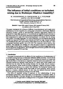
Figure 1. Schematic of the experimental facility showing the shock tube, the nozzle (N), suction duct (S), the reshock wall (RW), diaphragm (P), pressure transducers (marked +) and planar laser influenced fluorescence (PLIF) cameras. All dimensions are given in meters.

patterns after reshock are expected to be dependent upon the ICs [15]. It is possible that a reshock wave will drive the flow to a more turbulent state, with an associated tendency to isotropy that reduces the imprint of the ICs, although experimental evidence is lacking here. Using a reshock wall positioned at a fixed distance from the IC, we examine the effect of reshocking a varicose curtain and compare it with the reshocked structures from a sinuous curtain to show mean density differences between the two cases. Such measurements precede full turbulence measurements and become important in finding regions within curtains where turbulence statistics might become homogeneous.

Figure 2. Enlarged schematic of the test section showing camera positions, laser light sheet and the gas curtain.

0.1420 0.2540 0.1562

2. Experiment 0.2540 2.1. Experimental facility

0.5680

The experiments reported here are performed in a horizontal shock tube with a 3 in.2 cross section. The shock tube is operated with pressurized nitrogen as the driver gas and air as the driven fluid. The rupture of the diaphragm that separates the driver and the driven sections creates a Mach 1.2 shock wave that traverses the length of the tube to impinge upon a gas curtain that spans the test section (figure 1). The gas curtain is created by a gravity-driven flow of SF6 from a settling chamber through a flow straightening section connected to a nozzle fixed to the top wall of the shock tube. A suction manifold attached to the bottom of the shock tube below the nozzle is used to remove the flowing SF6 from the shock tube (figure 2). The modular nature of the nozzle flow section allows the easy swap of nozzles use to create initial conditions of various modal compositions (figure 3). The varicose mode is created by the diffusion of SF6 as it exits from a row of closely spaced cylinders (top of figure 3). The sinuous mode is created by diffusion of the flow as it exits from a row of closely spaced cylinders that are offset from their neighbors in the streamwise direction (middle of figure 3). The large-wavelength sinuous mode IC of the same amplitude as the sinuous mode but a different wavelength is produced by three rows of offset cylinders shaped as a sawtooth (bottom of figure 3). It should be emphasized that the cylinders are placed very close to one other to enhance the effect of diffusion, resulting in ICs and evolution patterns that are different from those that emerge upon shocking widely spaced cylinders [16]. The nozzles are manufactured using stereolithography and are designed to mitigate the oscillatory instabilities of the flowing curtain [14].

0.1562 0.5680

0.1420 0.0781

Figure 3. Three different nozzle configurations used in the present experiments: varicose mode (top), sinuous mode (middle) and the large-wavelength sinuous mode (bottom). The diffusion of SF6 in air creates a uniform gas layer with superimposed perturbations. Each nozzle configuration has the same total number of cylinders, of 0.1181 in diameter each, resulting in the same volume flow rate. All dimensions are given in inches.

The evolution of the flow is observed using a PLIF technique that involves seeding the flow with acetone vapor, generated by bubbling the SF6 through liquid acetone immersed in a bath of water maintained at 20 ◦ C. The acetone in the flow is excited by the output from a dual-head Gemini Nd-YAG laser operated at 266 nm. The emergent laser beam is shaped into a thin sheet of light of less than 0.5 mm thickness and is aligned parallel to the top wall, 20 mm below the nozzle exit. The broadband fluorescence of the acetone with a peak centered around 420 nm [17] is imaged using a pair of Apogee cameras (marked IC and DYN in figure 2). The CCD arrays in the IC and DYN cameras are operated to capture images with arrays of 728 × 490 and 1024 × 1024 pixels, providing effective resolutions of 46.4 and 54.4 µm, respectively. Both the cameras are equipped with a Tamron SP Macro lens fitted with sharp visible light interference filters centered around 532 nm with a full width at half maximum (FWHM) of 10 nm. 2

Phys. Scr. T132 (2008) 014013

B J Balakumar et al

Figure 4. PLIF image captured with the second laser pulse when the first laser pulse is timed to occur after (a, c) and before (b, d) shock impact on ICs at Mach 1.54 (a, b) and Mach 1.2 (c, d).

Trigger signals for the lasers, cameras and other electronics are generated from the output of four pressure transducers positioned along the shock tube and sampled at 10 million samples per second each. The first shock velocity was measured and controlled to within 416 ± 1m s−1 , whereas the reshock velocity with respect to the ground frame of reference was measured to be 324 ± 1m s−1 . Further details about the experimental setup are available elsewhere [14, 18].

The effects of the acetone bath temperature were eliminated by repeating the experiments in acetone baths that were maintained above and below the ambient temperature. In general, measurements at later times, higher Mach numbers and higher laser powers were observed to result in a more prominent imprint of this effect. These observations point to the necessity of being cautious while performing PLIF measurements of ICs immediately prior to shock impact in RM-unstable flows. The weak pressure waves created by the impigement of the laser beam on the gas curtain is one possible mechanism that will explain these observations. In all of the present experiments, the timing of the first laser pulse was chosen to be later than shock impact resulting in the elimination of this effect to within our ability to observe it.

2.2. Effect of measuring the IC with a laser pulse Laser-based techniques have been used for many decades now to generate experimental measurements on flows including RM flows. While the effect of the laser beam’s intrusion into the flow is generally negligible for most of the cases, there might be instances where the effect of the laser is non-negligible for the subsequent flow development. This is especially true in flows that have a tendency to amplify small perturbations during the course of its evolution, like the RM flows. Here, we document a case where the measurement of the IC with a laser pulse immediately prior to shock impact produces a development pattern that is slightly different from the pattern that develops in the absence of the laser pulse. To illustrate this effect, figure 4(a) shows the development of RM-unstable structures at Mach 1.54 with the first laser pulse timed to occur 100 µs after the shock wave has impacted the curtain, whereas figure 4(b) shows the dynamic image taken with the same nominal ICs in a run with the first laser pulse timed to occur less than 5 µs before shock impact. It is clear that a thickening of the bridge is observed in figure 4(b) relative to figure 4(a) (by comparing regions A and B for example), in addition to the development of a different mushroom pattern. It should be noted that the difference in shock speeds between these two shots was less than 0.2%, and that this effect was consistently repeatable over 20 shots for each case. Further, the modification of the mushroom development and the thickening of the bridge are also observed at Mach 1.2, as shown in figures 4(c) and (d). One might be led to suspect that the heating of the optics in the optical path of the laser by the first pulse might result in the observations shown in figure 4. However, by timing the first laser pulse to occur before and after shock impact, measurements were taken to confirm that this effect of the first laser pulse observed here was not an optical artifact. Next, the laser pulses were interchanged and the first laser switched off only to observe the same effect in both cases.

3. Discussion 3.1. Projectile structures due to shock focusing effects Complex transmission, reflection and refraction phenomena occur during the interaction of the shock wave with the diffuse density interfaces created by the gas curtain in the shock tube [3]. Due to the slower speed of the shock wave in SF6 in comparison to the ambient air, the planar shock wave quickly gets deformed as it is transmitted through the upstream interface of the curtain. This deformed shock wave induces accelerations within the curtain that are not entirely perpendicular to the plane of the shock wave resulting in the formation of cusp-like structures within each wavelength of the curtain [16]. The cusp-like structures develop further and eject material in the direction of the mean velocity, creating a spike of heavy material that protrudes out of the main RM mushroom structures. While these spikes are barely visible in the Mach 1.2 experiments, they become progressively stronger as the Mach number is increased [18]. A mushroom structure obtained using PLIF imaging at t = 115 µs after shock impact is shown in figure 5(a). The cusp described for a single cylinder in [16] is shown enlarged from the middle of the region marked with a square, where the spikes are not clearly visible. However, inverting the image and adjusting the contrast brings both the cusp (in the region A) and the spike (in the region B) into clear view (figure 5(b)). As the spike develops, the already small amount of material within the spike is dispersed over a larger volume, resulting in a progressively weaker PLIF signal strength with time. Yet, it is interesting that at a later time (t = 215 µs), the spike structures could still be observed, albeit at a low intensity 3

Phys. Scr. T132 (2008) 014013

B J Balakumar et al

Figure 5. Projectiles due to shock focusing: (a) a PLIF image of flow development at 115 µs upon shock by a Mach 1.54 shock wave with the cusp [16] region enlarged; (b) the same image in (a) inverted and color contrast adjusted to show the spike structures. (c) PLIF image of flow development at 215 µs showing no clear spike evidence, (d) the same image in (c) upon contrast adjustment shows the presence of the spike remnants resembling a reverse mushroom structure.

(figure 5(d)). Further, the tip of the spike in figure 5(b) is observed to be flat rather than pointed (marked B). It is not clear whether the flattened spike tips are mushroom structures that develop from the vorticity carried by the tips, or if they are created by the stagnation of the spike that has lost its momentum. In either case, in a multi-layered gas curtain [19], the perturbations induced by the impingement of the spike into adjacent layers modify the vortex interactions, and subsequently affect the flow evolution itself. These perturbations might be further amplified in the presence of a reshock. Finally, simulations thus far have not captured these spike structures in gas curtains [4, 5, 20], pointing to a potential lack of resolution in their computational domains. It remains an interesting challenge to capture the experimentally observed spikes in RM simulations, and analyze the structures for vorticity.

downstream perturbations are subjected to a phase inversion before reaching a state of monotonic perturbation growth, whereas the upstream perturbations grow immediately without any inversion (t = 45 µs). The growing perturbations follow a sinuous mode of growth (t = 190 µs) and remain spanwise periodic until the times investigated (t = 565 µs). The increase in the width of the instability is attributable to the velocity field (created by the row of counter-rotating vortices) that wraps the heavy gas material and concurrently drives the inter-vortex material away from the center of the vortices. The experimentally measured growth curves in this case follow the form of the equations in the model provided by [13], which assumes a row of equispaced counter-rotating point vortices. The development of the sinuous perturbation follows a more complex pattern as shown in figure 6(b). The sinuous nozzles were manufactured to test the existence of the opposite mushroom (OM) patterns predicted in numerical experiments. Readily apparent are the OM features predicted by the simulations of [5] at times t = 180–330 µs. One expects the vorticity to be deposited near the edges of the downstream regions that present a concave surface to the incoming shock wave (denoted by squares in figure 6). It appears that these edges (and regions of associated vorticity) are driven toward one another by the upstream vortices (point-vortex regions denoted by circles). As the deposited vortices approach each other, their self-induction becomes stronger and they are pushed out from the main structure eventually creating the downstream elements of the OM structures. The combined velocity field induced by the two rows of vortices compresses and stretches the concave regions into thin bridges that connect the mushroom structures spanwise.

3.2. Evolution of various ICs after first shock Time-series images showing the essential stages in the evolution of three different ICs are presented in figures 6 and 7. Figure 6(a) shows the evolution from a varicose perturbation, figure 6(b) shows the evolution from a sinuous interface, and figure 7 shows a limited dataset of evolution from a sinuous interface with a higher wavelength but the same amplitude as in (b). It should be noted that the perturbations in each of these ICs have a large amplitude comparable to the primary wavelength. The spanwise periodic development of the varicose perturbation after shock impact and the nonlinear development at late times without a readily apparent transition to turbulence are shown in figure 6(a). Detailed explanations are provided in [14, 18], but will be briefly reviewed here for completeness. Upon shock impact, the 4

Phys. Scr. T132 (2008) 014013

B J Balakumar et al

Figure 6. A comparison of RM-instability evolution for the (a) varicose and (b) sinuous IC configurations showing the concentration of vortices after first shock, and after reshock (last image in each time series). Numbers beside the images represent the times after first shock in microsecond. Arrow represents the direction of first shock.

The flow development in the case of the large-wavelength sinuous mode is shown in figure 7 at three different times along with the IC. A comparison of the evolution patterns presented in figures 6 and 7 shows that the flow emerging from

each of the ICs is dominated by the presence of concentrated regions of vorticity. The presence of various configurations of vortices implies that growth models for these kinds of flows should consider the interaction of the vortices with one other 5

Phys. Scr. T132 (2008) 014013

B J Balakumar et al

Figure 7. The evolution of RM-instability from an IC with large-wavelength sinuous perturbations after first shock. Numbers represent times after first shock in microseconds. The first shock moves from left to right.

in addition to their interaction with the surrounding fluid, especially when the vortex configuration is unstable.

The integration is executed using a 4th-order Runge–Kutta scheme with 460 time steps of 1 µs each. While this procedure is admittedly simple, it appears to capture the essential physics of the vortex-dominated flow. The results show that the downstream row of vortices get advected far more than the upstream row. Moreover, the directions of advection of the upstream and downstream vortex rows are opposite, resulting in a substantial growth rate increase due to advection. This self-advection becomes even more important in the case of reshock as the reshock wave encounters material that has been moved away from the main structure by the downstream vortex row. Thus, the width of the structure after first shock and the width after reshock are clearly dependent upon the vortex dynamics of the configuration that is created after the first shock. This connection between the reshocked turbulent structures and the vortex motions after first shock has seldom been explored or considered in turbulence models for RM flows. For further details about the analysis of the equilibrium, stability and motion of various vortex configurations, the interested reader is referred to [22, 23]. Based on the vortex model presented here, it is expected that the width of the structures in the sinuous configuration follows a linear increase with time.

3.3. Vortex dominated post-shock evolution The interaction of the first shock with the varicose IC results in the generation of a row of counter-rotating vortices (see figure 6(a) at t = 465 µs). A similar interaction with the sinuous curtain results in two rows of counter-rotating vortices (figure 6(b) at t = 180–330 µs). While the spacing between the positive and negative vortices in the varicose curtain is roughly equal to half the primary wavelength resulting in evenly spaced vortices, the spacing between the downstream counter-rotating vortex pairs in the sinuous mode is much lower than the primary wavelength. It is a well-known result that an infinite row of counter-rotating vortices that are not equispaced are not in equilibrium and, as a result, propel each other through the surrounding fluid [21] resulting in a mean velocity for the row as a whole. Hence, it is reasonable to expect that the downstream row of vortices in the sinuous mode propel themselves and the surrounding material through mutual vortex-pair induction, resulting in width amplification. Indeed, the basic equation of motion for a set of N -point vortices is given by [21, 22] as

3.4. IC dependence of mean density after reshock N 1 X 0β = , dt 2πι β=1 z α − z β

dz α∗

The clear separation between the upstream and downstream mushrooms at t = 580 µs in the evolution of the sinuous IC might lead one to suspect that the reshocked turbulent structure would exhibit clearly demarcated regions of material concentration corresponding to each row of vortex pairs. This would be in contrast to the varicose nozzle where most of the material is distributed in close proximity to the center of mass of the evolving structure. However, images of the reshocked curtain for each case, shown at the bottom of figure 6, paint a somewhat different picture. To quantify this effect, we calculate the streamwise variation in the mean density field at time, t = 630 µs after reshock. The mean density field is calculated by ensemble averaging the reshocked

(1)

where z α is the complex location of the vortex numbered α at a given time, t and 0α is its circulation. The trajectories of the vortices obtained from an integration of this equation for the sinuous mode are shown in figure 8. The integration is carried out using parameter values of λ = 3.6 mm, δ1 = 1.36 mm, δ2 = 0.82 mm, 01 = 02 = 0.04 m2 s−1 , wi = 2.68 mm and 40 quadruplets for the vortex model (notation used here is defined in figure 8(a)). The values of the parameters are chosen based on inspection of the image data at time, t = 120 µs. The circulation values are estimated from particle imaging velocimetry (PIV) measurements in related flows. 6

Phys. Scr. T132 (2008) 014013

B J Balakumar et al -2

0

x

x

2

4

6

-5

0

5

Figure 8. (a) A single cell from a periodic point-vortex model to describe the evolution of the sinuous curtain after the formation of the counter-rotating vortex double row; (b) computed trajectory of two rows of counter-rotating point vortices as they are advected by the cumulative velocity induced by all the surrounding vortices.

Normalized mean density differential

images from fifteen different experiments at time t = 1215–1230 µs after first shock. The variation of the density in the streamwise direction is then estimated by averaging the ensemble density field in the spanwise direction. Thus, the normalized density differential, (hρi(x) − hρ air i(x))/|hρi(x) − hρ air i(x)|max is estimated using the following equation (where brackets denote an ensemble average and overbars denote spanwise average): hρi(x) − hρ air i(x)

= |hρi(x) − hρ air i(x)|max R Pn air i=1 (ρi (x, y) − ρi (x, y))dy y R P n y i=1 (ρi (x, y) − ρiair (x, y))dy

.

(2)

max

1

0.8

0.6

S

0.4

0.2

0

The convergence of the statistics was tested using several different subsets from this ensemble of density fields. Based upon 100 different random permutations of eight images each, the maximum error in the estimate of the mean is estimated to be ±10%. In each of these cases, the shape of the curves remained similar to the mean curve presented here. Further, by using different window lengths during the averaging of the density in the spanwise direction, it was verified that the variations observed here are not artifacts of using a large window size but are features of the true ensemble statistics. The variation of the mean density differential in the streamwise direction for the varicose and sinuous curtain is shown in figure 9. For the varicose curtain (marked V), the mean density reaches a peak value near the center of the curtain and tapers off on either side of the peak. In contrast, for the sinuous curtain, a region of roughly constant mean density exists, despite the presence of two distinct regions of material in the pre-reshock structure (associated with the upstream and downstream vortex rows). Thus, it appears that the reshock has deposited energy that has rapidly mixed the previously distinct sets of structures. This constant-density region spans a distance of about 6 mm, which is about 25% of the total width. This observation suggests an attractive possibility for the variable-density turbulence researcher, viz the existence of well-mixed regions in thick curtains where the turbulence statistics might become spatially invariant.

V

80

85

90

95

100

Streamwise location (mm) Figure 9. Variation of the spanwise ensemble averaged normalized mean density differential profiles with streamwise location for the sinuous (S) and varicose (V) configuration gas layers.

4. Conclusions Destabilization of three ICs with different modal compositions show that the post-shock evolution of RM instability is dominated by concentrated regions of vorticity. A comparison of the development of the varicose and sinuous modes suggests that the dominant mechanisms driving the growth of the layer depend upon the stability of the vortex configuration created in the initial (post-shock) flow. In the case of a stable initial configuration of vortices (that emerges from shocking the varicose curtain, for example), the structure width will be dominated by the advection of material by the induced velocity field. However, in the case of an unstable initial configuration (sinuous curtain, for example), the vortices may self-induce to severely alter the initial vortex configuration and in conjunction with material advection, dramatically increase the layer width. The opposite-mushroom structures reported in numerical simulations [5] are observed experimentally for the first time. 7

Phys. Scr. T132 (2008) 014013

B J Balakumar et al

While these structures are prominent after first shock, their dual-layer signature is erased well after reshock in the sinuous case, resulting in substantial mixing and a resultant broad region of roughly constant mean density near the middle of the turbulent structure. The existence of this well-mixed region within the sinuous curtain where the turbulence statistics might remain spatially homogeneous in both the streamwise and spanwise directions will be the subject of future investigations.

[9] Zabusky N J, Ray J and Samtaney R 1995 Vortex models for the Richtmyer–Meshkov instability ed R Youngs, J Glimm and B Boyton Proc. 5th Int. workshop on Physics of Compressible Turbulent Mixing [10] Rikanati A, Alon U and Shvarts D 1998 Vortex model for the nonlinear evolution of the multimode Richtmyer–Meshkov instability at low Atwood numbers Phys. Rev. E 58 7410–18 [11] Zabusky N J 1999 Vortex paradigm for accelerated inhomogeneous flows: visiometrics for the Rayleigh–Taylor and Richtmyer–Meshkov environments Ann. Rev. Fluid Mech. 31 495–536 [12] Peng G Z, Zabusky N J and Zhang S 2003 Vortex-accelerated secondary baroclinic vorticity deposition and late-intermediate time dynamics of a two-dimensional Richtmyer-Meshkov interface Phys. Fluids 15 3730–44 [13] Jacobs J W, Jenkins D G, Klein D L and Benjamin R F 1995 Nonlinear growth of the shock-accelerated instability of a thin fluid layer J. Fluid Mech. 295 23–42 [14] Balakumar B J, Orlicz G, Tomkins C and Prestridge K 2008 Simultaneous PIV/PLIF measurements of Richtmyer–Meshkov instability growth in a gas curtain with and without reshock [15] Rightley P M, Vorobieff P, Martin R and Benjamin R F 1999 Experimental observations of the mixing transition in a shock-accelerated gas curtain Phys. Fluids 11 186–200 [16] Kumar S, Orlicz G, Tomkins C, Goodenough C, Prestridge K, Vorobieff P and Benjamin R 2005 Stretching of material lines in shock-accelerated gaseous flows Phys. Fluids 17 082107 [17] Lozano A, Yip B and Hanson R K 1992 Acetone: a tracer for concentration measurements in gaseous flows by planar laser-induced fluorescence Exp. Fluids 13 369–76 [18] Orlicz G 2007 Shock Driven Instabilities in a varicose, heavy-gas curtain: Mach number effects Master’s Thesis University of New Mexico, Albuquerque [19] Mikaelian K O 1983 Time evolution of density perturbations in accelerating stratified fluids Phys. Rev. A 28 1637 [20] Kamm J R, Rider W, Tomkins C D, Zoldi C, Prestridge K, Marr-Lyon M, Rightley P, Vorobieff P and Benjamin R 2002 Statistical comparison between experiments and numerical simulations of two shock-accelerated gas cylinders Technical Report Los Alamos National Laboratory [21] Lamb H 1932 Hydrodynamics (New York: Dover) [22] Aref H 1995 On the equilibrium and stability of a row of point vortices J. Fluid Mech. 290 167–81 [23] Aref H 1983 Integrable, chaotic and turbulent vortex motion in two-dimensional flows Annu. Rev. Fluid Mech. 15 345–89

Acknowledgments We acknowledge the support of the Department of Energy during this research. The help provided by Dr Devesh Ranjan during some of the data acquisition is gratefully acknowledged.

References [1] Jacobs J W, Klein D L, Jenkins D G and Benjamin R F 1993 Instability growth patterns of a shock-accelerated thin fluid layer Phys. Rev. Lett. 70 583–6 [2] Budzinski J M, Benjamin R F and Jacobs J W 1994 Influence of initial conditions on the flow patterns of a shock-accelerated thin fluid layer Phys. Fluids 6 3510–2 [3] Budzinski J M, Benjamin R F and Jacobs J W 1995 An experimental investigation of shock-accelerated heavy gas layers Technical Report Los Alamos National Laboratory [4] Baltrusaitis R M, Gittings M L, Weaver R P, Benjamin R F and Budzinski J M 1996 Simulation of shock-generated instabilities Phys. Fluids 8 2471–83 [5] Mikaelian K O 1996 Numerical simulations of Richtmyer–Meshkov instabilities in finite-thickness fluids layers Phys. Fluids 8 1269–92 [6] Rider W and Kamm J R 2000 Impact of numerical integration on gas curtain simulations Technical Report LANL [7] Prestridge K P, Vorobieff P, Rightley P M and Benjamin R F 2001 PIV measurements of a shock-accelerated fluid instability ed K Takayama, T Saito, H Kleine and E Timofeev Proceedings of SPIE 4183 [8] Hawley J F and Zabusky N J 1989 Vortex paradigm for shock-accelerated density-stratified interfaces Phys. Rev. Lett. 63 1241–4

8