12th WSEAS International Conference on SYSTEMS, Heraklion, Greece, July 22-24, 2008
Impact of Initial Conditions and Voltage Source on the Initiation of Fundamental Frequency Ferroresonance KRUNO MILIČEVIĆ, IVAN RUTNIK - Faculty of Electrical Engineering, Osijek IGOR LUKAČEVIĆ - HEP-Transmission system operator Ltd, Osijek CROATIA http://www.etfos.hr; http://www.hep.hr Abstract: The impact of initial conditions on the initiation of fundamental frequency ferroresonance is investigated. The investigation is carried out by simulating the behaviour of the mathematical model of ferroresonant circuit realized in the laboratory. The initiation of fundamental frequency ferroresonance is investigated by varying the values of phase angle and amplitude of voltage source in order to incite the ferroresonance. Thereby, the initial conditions are varied within a practically possible range of initial values of transformer voltage and transformer flux linkage. Keywords: Ferroresonance, Iron-cored reactor, Bifurcation diagram, Chaos, Nonlinear circuits
1 Introduction
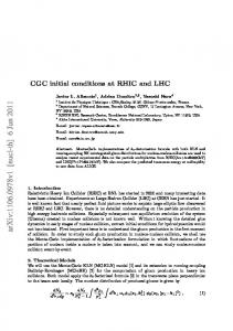
power system for the ferroresonance case studies. An example of ferroresonance in three phase transmission system is shown on Fig. 3.
The simple electrical circuit in which ferroresonant oscillation can occur is a circuit which comprises a linear capacitor in series with a nonlinear coil, driven by a sine-wave voltage source, Fig. 1. The nonlinearity of the coil comes from the nonlinear magnetization characteristic of the iron core. The usual electrical model of the nonlinear coil is a nonlinear reactor described by iL(ϕ) characteristic in parallel with a nonlinear resistor described by iR(uL) characteristic, Fig. 2.
Figure 3. Ferroresonance in three phase system
The nonlinear inductances represent iron core coils of unloaded three phase power transformer and the capacitance (Cm, CZ) represents capacitance of long transmission line (or HV underground cable). The ferroresonance occurs because of the malfunction of one pole of HV circuit breaker. The Fig. 1 shows the equivalent circuit where Figure 1. Ferroresonant circuit
u = (u 2 + u3 )
Cm 2C m + C Z
(1)
C = 2C m + C Z
More practical examples are described in the literature [1]. Ferroresonant circuit is a nonlinear dynamical system and as such its behaviour can be analyzed using methods available in chaos theory. Three basic types of ferroresonance have been identified [2, 3]: the fundamental frequency ferroresonance, subharmonic ferroresonance, where the period of oscillation is an integral multiple of the period of the
Figure 2. Model of nonlinear coil
The nonlinear coil is realized either as a winding of the unloaded iron-cored transformer or as a winding of the iron-cored reactor without air gap. The analyzed circuit is a laboratory model, but in praxis it is a simplest physical model of a large electrical
Corresponding author. K. Milicevic is with the Faculty of Electrical Engineering, Osijek, Croatia (e-mail:
[email protected]). Tel: 00385912246021; Fax: 0038531224708.
ISBN: 978-960-6766-83-1
64
ISSN: 1790-2769
12th WSEAS International Conference on SYSTEMS, Heraklion, Greece, July 22-24, 2008
supply system, and chaotic ferroresonance, in which the oscillations appear to be random. From engineering point of view it is important to predict the bifurcation points, i.e. the values of source amplitude at which the change of steady-state responses takes place. Computer simulation is an inexpensive but powerful tool for this task, [4-7] and it will be used to investigate impact of initial conditions at source amplitude values that could incite the ferroresonance.
apparent power of 200 VA and for the nominal primary voltage of 30 V. The core was strip-wounded, made of Ni-Fe alloy (Trafoperm N3). The autotransformer of 10 kVA nominal apparent power was used as a variable voltage source in all experiments. The magnetization characteristic iL (ϕ ) and the iron-core losses R are derived from measured P-U and U-I characteristic of the nonlinear coil [8]. Thereby, the resistor R is supposed to be linear.
2 Mathematical model of the ferroresonant circuit
3 Simulation results In order to determine the impact of initial conditions on the initiation of fundamental frequency ferroresonance Eq. (2) was solved using the commercially available software package MATLAB/Simulink employing the Dormand-Prince method which is the default solver used by Simulink for models with continuous states [9]. Preliminary simulations were carried out by varying the values of initial conditions of voltage u L and flux linkage ϕ : ⎛m ⎞ (4) u L (0) m = 2Uˆ ⎜ − 1⎟; m = 0,1,...,100 ⎝ 50 ⎠ 2Uˆ ⎛ n ⎞ (5) ϕ (0) n = ⎜ − 1⎟; n = 0,1,...,100 ω ⎝ 50 ⎠ The simulations were carried out for eight different values of the phase shift α: π (6) α = k ; k = 0,1,...,7 4 and for value of source amplitude Uˆ = 0.7 . All other
The time domain behaviour of the basic ferroresonant circuit of Fig. 2 can be described by the following differential equations: dϕ = u L = Uˆ sin(ωt + α ) − uC dt duC 1 ⎡ uC ⎤ = ⎢ + iL (ϕ) ⎥ dt C⎣R ⎦
(2)
The variables and parameters of the ferroresonant circuit can also be expressed in a relation to base quantities; that is, in a per-unit system: ϕ=ϕ
u ω i Uˆ ; uC = C ; τ = ωt ; iL = L ;Uˆ = U ref U ref I ref U ref
Reference values U ref = 31.2V; I ref = 0.19A
parameters were fixed. Theoretically, both initial conditions, as well as phase shift value α, could be equal to an indefinite number of different values inside the above-defined boundaries. In order to determine the impact of these parameters and, at the same time, to limit the range and duration of investigation to a reasonably practical level, they were changed in above-defined fixed steps (4-6) within the defined range. These combinations result into 10201 different sets of initial values and hence as many steady-state solutions for each value of voltage source phase. The dependence of the steady-state solution and consequently the initiation of fundamental frequency ferroresonance on initial conditions are depicted in Figs. 4 in what could be called a 2-parameter bifurcation diagram for eight different phase shift values and for source amplitude value Uˆ = 0.7 . For easier visualization the diagrams were
parameters of the model ω =1 ; C =1 ; R =
uL =2 iR
as well as the polynomial form of the magnetization nonlinearity: iL (ϕ) = f (ϕ)sign(ϕ) f (ϕ) = 0.034 ⋅ ϕ2 + 5.54 ⋅10−3 ⋅ ϕ20 + 1.05 ⋅10−5 ⋅ ϕ38
(3)
derive from the model of the ferroresonant circuit realized in the laboratory that is composed of the linear capacitor C=20 μF and the nonlinear coil. The primary winding of the toroidal iron-cored two-winding transformer was used as a nonlinear coil. The transformer was designed for the nominal
ISBN: 978-960-6766-83-1
65
ISSN: 1790-2769
12th WSEAS International Conference on SYSTEMS, Heraklion, Greece, July 22-24, 2008
ϕ (0) n are qualitatively equal to the steady-state solutions shown on Figs. 4e-4h, respectively, obtained for initial values − u L (0) m and − ϕ (0) n , i.e. the Figs. 4a-4d are symmetric to the Fig.4e-4h, respectively, with respect to the angle π. The presented results are obtained only for one value of source amplitude value and eight different values of phase angle from the range of possible values. To cover a wider range of source voltage values that could incite the ferroresonance, the 2-parameter bifurcation diagrams are obtained for following values of source amplitude also:
constructed using colour coded squares where different colours were employed to represent different steady-state solution: normal sinusoidal steady-state, fundamental frequency ferroresonance
Uˆ = 0.1⋅ l + 0.7; l = 1, 2,3 Thereby, according to results shown on Fig. 4, i.e. because of the rotational symmetry, there is no need to obtain 2-parameter bifurcation diagrams for phase shift values α ≥ π . Thus, the 2-parameter bifurcation diagrams were obtained for following phase shift values only: π α=k ; k = 0,1, 2,3 4 Values of initial conditions of voltage u L and flux linkage ϕ where varied as in the preliminary simulations (4, 5). All other parameters were fixed. Fig. 5 shows obtained 2-parameter bifurcation diagrams.
Figure 4. 2-parameter bifurcation diagrams for source amplitude value Uˆ = 0.7
For example, the square at ( ϕ (0)14 , u L (0)89 ) on Fig.4a represents normal sinusoidal response for the initial conditions of: 36 2Uˆ ϕ (0)14 = − = −1.426 50 ω and 39 u L (0)89 = 2Uˆ = 1.544 50 Resultant steady-state solution types shown on Fig. 4 indicate the rotational movement of the area corresponding to the normal sinusoidal steady-state (“black” area) in a clockwise direction. It should be noted that for the steady-state results obtained under phase angle α and for those obtained under α+π there is a rotational symmetry in the diagrams shown in Fig. 4a and Fig. 4e. Namely, the types of steady-state solutions shown on Figs. 4a-4d obtained for initial values u L (0) m and
ISBN: 978-960-6766-83-1
a) Uˆ = 0.8
66
ISSN: 1790-2769
12th WSEAS International Conference on SYSTEMS, Heraklion, Greece, July 22-24, 2008
The ferroresonance in the electrical power system is an undesirable phenomenon often with harmful consequence. During the electrical power system design process, all possible initial conditions must be considered to identify potentially unstable states and to avoid the ferroresonance. Future work will widen the investigation of impact of initial conditions on the initiation of a subharmonic and chaotic ferroresonance. References: [1] IEEE Working Group, "Modelling and analysis guidelines for slow transients – part III: The study of ferroresonance," IEEE Transactions on Power Delivery, Vol. 15, No. 1, pp. 255-265, 2001. [2] C. Kieny, “Application of the bifurcation theory in studying and understanding the global behavior of a ferroresonant electric power circuit,” IEEE Trans. Power Delivery, Vol. 6, pp. 866–872, 1991. [3] S. Mozaffari, S. Henschel, and A. C. Soudack, “Chaotic ferroresonance in power transformers,” Proc. IEE Generation, Transmission Distrib., Vol. 142, No. 3, pp. 247– 250, 1995. [4] J.R.Marti, A.C.Soudack, "Ferroresonance in power systems: Fundamental solutions," IEE Proceedings-C, Vol. 138, No. 4, pp. 321-329, 1991. [5] B.Lee, V.Ajjarapu, "Period-doubling route to chaos in an electrical power system," IEE Proceedings-C, Vol. 140, No. 6, pp. 490-496, 1993. [6] A.E.A. Araujo, A.C.Soudack, J.R.Marti, "Ferroresonance in power systems: Chaotic behaviour," IEE Proceedings-C, Vol. 140, No. 3, pp. 237-240, 1993. [7] Z. Emin, B. A. T. Al Zahawi, D. W. Auckland and Y.K. Tong, "Ferroresonance in Electromagnetic Voltage Transformers: A Study Based on Nonlinear Dynamics," IEE Proc.Generation, Transmission, Distribution, Vol. 144, No. 4, July 1997, pp. 383-387. [8] I.Flegar, D.Fischer, D.Pelin "Identification of chaos in a ferroresonant circuit," IEE Power Tech '99 Conference, Budapest, Hungary, August 29-September 2, 1999; pp. 1-5, 1999. [9] The MathWorks – MATLAB and Simulink for Technical Computing. 4th of January 2008. http://www.mathworks.com/access/helpdesk/hel p/toolbox/simulink/index.html?/access/helpdesk /help/toolbox/simulink/ug/f11-69449.html .
b) Uˆ = 0.9
c) Uˆ = 1.0 Figure 5. 2-parameter bifurcation diagrams for source amplitude values Uˆ = 0.8, 0.9, 1.0
4 Conclusions By fixing the value of source voltage amplitude and varying the initial condition values of transformer voltage and flux linkage for eight different values of phase angle of voltage source (αk=k·π/4; k=0, …, 7), the initial conditions have been shown to have a clear definite impact on the initiation of fundamental frequency ferroresonance. Furthermore, the steadystates obtained for values αk=k·π/4, (k = 0, 1, 2, 3) are symmetric to the steady-states obtained for values αk=k·π/4, (k = 4, 5, 6, 7) respectively, with respect to the angle π. Therefore, to investigate the impact of initial conditions on the initiation of fundamental frequency ferroresonance, it is necessary to carry out the simulations for values of voltage source phase 0 ≤ α < π only. By increasing the source voltage amplitude, the area of ferroresonant steady-states on 2-parameter bifurcation diagrams increased also.
ISBN: 978-960-6766-83-1
67
ISSN: 1790-2769